Gmsh 
Christophe Geuzaine and Jean-François Remacle
Gmsh is an automatic 3D finite element mesh generator with build-in pre- and post-processing facilities. This is the Gmsh Reference Manual for Gmsh 5.0.0 (development version) (April 24, 2026).
Table of Contents
- Obtaining Gmsh
- Copying conditions
- Reporting a bug
- 1 Overview of Gmsh
- 2 Gmsh tutorial
- 2.1
t1: Geometry basics, elementary entities, physical groups - 2.2
t2: Transformations, extruded geometries, volumes - 2.3
t3: Extruded meshes, ONELAB parameters, options - 2.4
t4: Built-in functions, holes in surfaces, annotations, entity colors - 2.5
t5: Mesh sizes, macros, loops, holes in volumes - 2.6
t6: Transfinite meshes, deleting entities - 2.7
t7: Background meshes - 2.8
t8: Post-processing, image export and animations - 2.9
t9: Plugins - 2.10
t10: Mesh size fields - 2.11
t11: Unstructured quadrangular meshes - 2.12
t12: Cross-patch meshing with compounds - 2.13
t13: Remeshing an STL file without an underlying CAD model - 2.14
t14: Homology and cohomology computation - 2.15
t15: Embedded points, lines and surfaces - 2.16
t16: Constructive Solid Geometry, OpenCASCADE geometry kernel - 2.17
t17: Anisotropic background mesh - 2.18
t18: Periodic meshes - 2.19
t19: Thrusections, fillets, pipes, mesh size from curvature - 2.20
t20: STEP import and manipulation, geometry partitioning - 2.21
t21: Mesh partitioning - 2.22
x1: Geometry and mesh data - 2.23
x2: Mesh import, discrete entities, hybrid models, terrain meshing - 2.24
x3: Post-processing data import: list-based - 2.25
x4: Post-processing data import: model-based - 2.26
x5: Additional geometrical data: parametrizations, normals, curvatures - 2.27
x6: Additional mesh data: integration points, Jacobians and basis functions - 2.28
x7: Additional mesh data: internal edges and faces
- 2.1
- 3 Gmsh graphical user interface
- 4 Gmsh command-line interface
- 5 Gmsh scripting language
- 6 Gmsh application programming interface
- 6.1 Namespace
gmsh: top-level functions - 6.2 Namespace
gmsh/option: option handling functions - 6.3 Namespace
gmsh/model: model functions - 6.4 Namespace
gmsh/model/mesh: mesh functions - 6.5 Namespace
gmsh/model/mesh/field: mesh size field functions - 6.6 Namespace
gmsh/model/geo: built-in CAD kernel functions - 6.7 Namespace
gmsh/model/geo/mesh: built-in CAD kernel meshing constraints - 6.8 Namespace
gmsh/model/occ: OpenCASCADE CAD kernel functions - 6.9 Namespace
gmsh/model/occ/mesh: OpenCASCADE CAD kernel meshing constraints - 6.10 Namespace
gmsh/view: post-processing view functions - 6.11 Namespace
gmsh/view/option: view option handling functions - 6.12 Namespace
gmsh/algorithm: raw algorithms - 6.13 Namespace
gmsh/plugin: plugin functions - 6.14 Namespace
gmsh/graphics: graphics functions - 6.15 Namespace
gmsh/fltk: FLTK graphical user interface functions - 6.16 Namespace
gmsh/parser: parser functions - 6.17 Namespace
gmsh/onelab: ONELAB server functions - 6.18 Namespace
gmsh/logger: information logging functions
- 6.1 Namespace
- 7 Gmsh options
- 8 Gmsh mesh size fields
- 9 Gmsh plugins
- 10 Gmsh file formats
- Appendix A Compiling the source code
- Appendix B Information for developers
- Appendix C Frequently asked questions
- Appendix D Version history
- Appendix E Copyright and credits
- Appendix F License
- Concept index
- Syntax index
Obtaining Gmsh 
The source code and pre-compiled binary versions of Gmsh (for Windows, macOS and Linux) can be downloaded from https://gmsh.info. Gmsh packages are also directly available in various Linux and BSD distributions (Debian, Fedora, Ubuntu, FreeBSD, ...).
If you use Gmsh, we would appreciate that you mention it in your work by citing the following paper: C. Geuzaine and J.-F. Remacle, Gmsh: a three-dimensional finite element mesh generator with built-in pre- and post-processing facilities. International Journal for Numerical Methods in Engineering, Volume 79, Issue 11, pages 1309-1331, 2009. A preprint of that paper as well as other references and the latest news about Gmsh development are available on https://gmsh.info.
Copying conditions 
Gmsh is free software; this means that everyone is free to use it and to redistribute it on a free basis. Gmsh is not in the public domain; it is copyrighted and there are restrictions on its distribution, but these restrictions are designed to permit everything that a good cooperating citizen would want to do. What is not allowed is to try to prevent others from further sharing any version of Gmsh that they might get from you.
Specifically, we want to make sure that you have the right to give away copies of Gmsh, that you receive source code or else can get it if you want it, that you can change Gmsh or use pieces of Gmsh in new free programs, and that you know you can do these things.
To make sure that everyone has such rights, we have to forbid you to deprive anyone else of these rights. For example, if you distribute copies of Gmsh, you must give the recipients all the rights that you have. You must make sure that they, too, receive or can get the source code. And you must tell them their rights.
Also, for our own protection, we must make certain that everyone finds out that there is no warranty for Gmsh. If Gmsh is modified by someone else and passed on, we want their recipients to know that what they have is not what we distributed, so that any problems introduced by others will not reflect on our reputation.
The precise conditions of the license for Gmsh are found in the General Public License that accompanies the source code (see License). Further information about this license is available from the GNU Project webpage https://www.gnu.org/copyleft/gpl-faq.html. Detailed copyright information can be found in Copyright and credits.
If you want to integrate parts of Gmsh into a closed-source software, or want to sell a modified closed-source version of Gmsh, you will need to obtain a different license. Please contact us directly for more information.
Reporting a bug 
If, after reading this reference manual, you think you have found a bug in Gmsh, please file an issue on https://gitlab.onelab.info/gmsh/gmsh/issues. Provide as precise a description of the problem as you can, including sample input files that produce the bug. Don’t forget to mention both the version of Gmsh and your operation system.
See Frequently asked questions, and the bug tracking system to see which problems we already know about.
1 Overview of Gmsh 
Gmsh is a three-dimensional finite element mesh generator with a build-in CAD engine and post-processor. Its design goal is to provide a fast, light and user-friendly meshing tool with parametric input and flexible visualization capabilities.
Gmsh is built around four modules (geometry, mesh, solver and post-processing), which can be controlled with the graphical user interface (GUI; see Gmsh graphical user interface), from the command line (see Gmsh command-line interface), using text files written in Gmsh’s own scripting language (.geo files; see Gmsh scripting language), or through the C++, C, Python, Julia and Fortran application programming interface (API; see Gmsh application programming interface).
A brief description of the four modules is given hereafter, before an overview of what Gmsh does best (... and what it is not so good at), and some practical information on how to install and run Gmsh on your computer.
- Geometry module
- Mesh module
- Solver module
- Post-processing module
- What Gmsh is pretty good at …
- … and what Gmsh is not so good at
- Installing and running Gmsh on your computer
1.1 Geometry module 
A model in Gmsh is defined using its Boundary Representation (BRep): a volume is bounded by a set of surfaces, a surface is bounded by a series of curves, and a curve is bounded by two end points. Model entities are topological entities, i.e., they only deal with adjacencies in the model, and are implemented as a set of abstract topological classes. This BRep is extended by the definition of embedded, or internal, model entities: internal points, curves and surfaces can be embedded in volumes; and internal points and curves can be embedded in surfaces.
The geometry of model entities can be provided by different CAD
kernels. The two default kernels interfaced by Gmsh are the
built-in kernel and the OpenCASCADE kernel. Gmsh does not
translate the geometrical representation from one kernel to another, or
from these kernels to some neutral representation. Instead, Gmsh
directly queries the native data for each CAD kernel, which avoids data
loss and is crucial for complex models where translations invariably
introduce issues linked to slightly different representations. Selecting
the CAD kernel in .geo scripts is done with the SetFactory
command (see Geometry scripting commands), while in the Gmsh API the
kernel appears explicitly in all the relevant functions from the
gmsh/model namespace, with geo or occ prefixes for
the built-in and OpenCASCADE kernel, respectively (see Namespace gmsh/model: model functions).
Entities can either be built in a bottom-up manner (first points, then curves, surfaces and volumes) with the built-in and OpenCASCADE kernels, or in a top-down constructive solid geometry fashion (solids on which boolean operations are performed) with the OpenCASCADE kernel. Both methodologies can also be combined. Finally, groups of model entities (called “physical groups”) can be defined, based on the elementary geometric entities. (See Elementary entities vs. physical groups, for more information about how physical groups affect the way meshes are saved.)
Both model entities (also referred to as “elementary entities”) and physical groups are uniquely defined by a pair of integers: their dimension (0 for points, 1 for curves, 2 for surfaces, 3 for volumes) and their tag, a strictly positive global identification number. Entity and group tags are unique per dimension:
- each point must possess a unique tag;
- each curve must possess a unique tag;
- each surface must possess a unique tag;
- each volume must possess a unique tag.
Zero or negative tags are reserved by Gmsh for internal use.
Model entities can be manipulated and transformed in a variety of ways within the geometry module, but operations are always performed directly within their respective CAD kernels. As explained above, there is no common internal geometrical representation: rather, Gmsh directly performs the operations (translation, rotation, intersection, union, fragments, ...) on the native geometrical representation using each CAD kernel’s own API. In the same philosophy, models can be imported in the geometry module through each CAD kernel’s own import mechanisms. For example, by default Gmsh imports STEP and IGES files through OpenCASCADE, which will lead to the creation of model entities with an internal OpenCASCADE representation. Models represented with the built-in CAD kernel can be serialized to disk by exporting them as .geo_unrolled files, while models contructed with the OpenCASCADE kernel can be serialized as .brep or .xao files.
The Gmsh tutorial, starting with t1: Geometry basics, elementary entities, physical groups, is the best place to
learn how to use the geometry module: it contains examples of increasing
complexity based on both the built-in and the OpenCASCADE kernel. Note
that many features of the geometry module can be used interactively in
the GUI (see Gmsh graphical user interface), which is also a good
way to learn about both Gmsh’s scripting language and the API, as
actions in the geometry module automatically append the related command
in the input script file, and can optionally also generate input for the
languages supported by the API (see the
General.ScriptingLanguages option; this is still work-in-progress
as of Gmsh 4.14.)
In addition to CAD-type geometrical entities, whose geometry is provided
by a CAD kernel, Gmsh also supports discrete model entities,
which are defined by a mesh (e.g. STL). Gmsh does not perform
geometrical operations on such discrete entities, but they can be
equipped with a geometry through a so-called “reparametrization”
procedure1. The parametrization is then
used for meshing, in exactly the same way as for CAD entities. See
t13: Remeshing an STL file without an underlying CAD model for an example.
1.2 Mesh module 
A finite element mesh of a model is a tessellation of its geometry by simple geometrical elements of various shapes (in Gmsh: lines, triangles, quadrangles, tetrahedra, prisms, hexahedra and pyramids), arranged in such a way that if two of them intersect, they do so along a face, an edge or a node, and never otherwise. This defines a so-called conformal mesh. The mesh module implements several algorithms to generate such meshes automatically. By default, meshes produced by Gmsh are considered as unstructured, even if they were generated in a structured way (e.g., by extrusion). This implies that the mesh elements are completely defined simply by an ordered list of their nodes, and that no predefined ordering relation is assumed between any two elements.
In order to guarantee the conformity of the mesh, mesh generation is performed in a bottom-up flow: curves are discretized first; the mesh of the curves is then used to mesh the surfaces; then the mesh of the surfaces is used to mesh the volumes. In this process, the mesh of an entity is only constrained by the mesh of its boundary, unless entities of lower dimensions are explicitly embedded in entities of higher dimension. For example, in three dimensions, the triangles discretizing a surface will be forced to be faces of tetrahedra in the final 3D mesh only if the surface is part of the boundary of a volume, or if that surface has been explicitly embedded in the volume. This automatically ensures the conformity of the mesh when, for example, two volumes share a common surface. Mesh elements are oriented according to the geometrical orientation of the underlying entity. Every meshing step is constrained by a mesh size field, which prescribes the desired size of the elements in the mesh. This size field can be uniform, specified by values associated with points in the geometry, or defined by general mesh size fields (for example related to the distance to some boundary, to a arbitrary scalar field defined on another mesh, etc.): see Gmsh mesh size fields. For each meshing step, all structured mesh directives are executed first, and serve as additional constraints for the unstructured parts. (The generation and handling of conformal meshes has important consequences on how meshes are stored internally in Gmsh, and how they are accessed through the API: see Gmsh application programming interface.)
Gmsh’s mesh module regroups several 1D, 2D and 3D meshing algorithms:
- The 2D unstructured algorithms generate triangles and/or quadrangles (when recombination commands or options are used). The 3D unstructured algorithms generate tetrahedra, or tetrahedra and pyramids (when the boundary mesh contains quadrangles).
- The 2D structured algorithms (transfinite and extrusion) generate triangles by default, but quadrangles can be obtained by using the recombination commands or options. The 3D structured algorithms generate tetrahedra, hexahedra, prisms and pyramids, depending on the type of the surface meshes they are based on.
All meshes can be subdivided to generate fully quadrangular or fully
hexahedral meshes with the Mesh.SubdivisionAlgorithm option
(see Mesh options).
- Choosing the right unstructured algorithm
- Specifying mesh element sizes
- Elementary entities vs. physical groups
1.2.1 Choosing the right unstructured algorithm 
Gmsh provides a choice between several 2D and 3D unstructured algorithms. Each algorithm has its own advantages and disadvantages.
For all 2D unstructured algorithms a Delaunay mesh that contains all the points of the 1D mesh is initially constructed using a divide-and-conquer algorithm2. Missing edges are recovered using edge swaps3. After this initial step several algorithms can be applied to generate the final mesh:
- The “MeshAdapt” algorithm4 is based on local mesh modifications. This technique makes use of edge swaps, splits, and collapses: long edges are split, short edges are collapsed, and edges are swapped if a better geometrical configuration is obtained.
- The “Delaunay” algorithm is inspired by the work of the GAMMA team at INRIA5. New points are inserted sequentially at the circumcenter of the element that has the largest adimensional circumradius. The mesh is then reconnected using an anisotropic Delaunay criterion.
- The “Frontal-Delaunay” algorithm is inspired by the work of S. Rebay6.
- Other experimental algorithms with specific features are also available. In particular, “Frontal-Delaunay for Quads”7 is a variant of the “Frontal-Delaunay” algorithm aiming at generating right-angle triangles suitable for recombination; and “BAMG”8 allows to generate anisotropic triangulations.
For very complex curved surfaces the “MeshAdapt” algorithm is the most robust. When high element quality is important, the “Frontal-Delaunay” algorithm should be tried. For very large meshes of plane surfaces the “Delaunay” algorithm is the fastest; it usually also handles complex mesh size fields better than the “Frontal-Delaunay”. When the “Delaunay” or “Frontal-Delaunay” algorithms fail, “MeshAdapt” is automatically triggered. The “Automatic” algorithm uses “Delaunay” for plane surfaces and “MeshAdapt” for all other surfaces.
Several 3D unstructured algorithms are also available:
- The “Delaunay” algorithm is split into three separate steps. First, an initial mesh of the union of all the volumes in the model is performed, without inserting points in the volume. The surface mesh is then recovered using H. Si’s boundary recovery algorithm Tetgen/BR. Then a three-dimensional version of the 2D Delaunay algorithm described above is applied to insert points in the volume to respect the mesh size constraints.
- The “Frontal” algorithm uses J. Schoeberl’s Netgen algorithm 9.
- The “HXT” algorithm10 is a new efficient and parallel reimplementaton of the Delaunay algorithm.
- Other experimental algorithms with specific features are also available. In particular, “MMG3D”11 allows to generate anisotropic tetrahedralizations.
The “Delaunay” algorithm is currently the most robust and is the only one that supports the automatic generation of hybrid meshes with pyramids. Embedded model entities and general mesh size fields (see Specifying mesh element sizes) are currently only supported by the “Delaunay” and “HXT” algorithms.
When Gmsh is configured with OpenMP support (see Compiling the source code), most of the meshing steps can be performed in parallel:
- 1D and 2D meshing is parallelized using a coarse-grained approach, i.e. curves (resp. surfaces) are each meshed sequentially, but several curves (resp. surfaces) can be meshed at the same time.
- 3D meshing using HXT is parallelized using a fine-grained approach, i.e. the actual meshing procedure for a single volume is done is parallel.
The number of threads can be controlled with the -nt flag on the
command line (see Gmsh command-line interface), or with the
General.NumThreads, Mesh.MaxNumThreads1D,
Mesh.MaxNumThreads2D and Mesh.MaxNumThreads3D options (see
General options and Mesh options).
1.2.2 Specifying mesh element sizes 
To determine the size of mesh elements, Gmsh locally computes the minimum of
- the size of the model bounding box;
- if
Mesh.MeshSizeFromPointsis set, the mesh size specified at geometrical points; - if
Mesh.MeshSizeFromCurvatureis positive, the mesh size based on the curvature of the curves and surfaces (the specified value is the number of elements per 2 Pi radians); - the background mesh size field, expressed as a combination of mesh size
fields (see Gmsh mesh size fields):
Boxfields specify the size inside and outside of a parallelepipedic region;Distancefields specify the size according to the distance to model entities;MathEvalfields specify the size using an explicit mathematical function;PostViewfields specify an explicit background mesh in the form of a scalar post-processing view (see Post-processing module, and Gmsh file formats) in which the nodal values represent the target sizes. This method is very general but it requires a first (usually rough) mesh and a way to compute the target sizes on this mesh (usually through an error estimation procedure, e.g. in an iterative process of mesh adaptation);Extendfields compute an extension of the sizes from a given boundary entity inside the enclosed surfaces or volumes;MinandMaxfields specify the size as the minimum or maximum of the sizes computed using other fields;- …
- any per-entity mesh size constraint.
Using the Gmsh API, this value can then be further modified using a C++,
C, Python, Julia or Fortran mesh size callback function provided via
gmsh/model/mesh/setSizeCallback (see Namespace gmsh/model/mesh: mesh functions).
The resulting value is then constrained in the interval
[Mesh.MeshSizeMin, Mesh.MeshSizeMax] (which can also be
provided on the command line with -clmin and -clmax) and
multiplied by Mesh.MeshSizeFactor (-clscale on the command
line).
Boundary mesh sizes are automatically interpolated during mesh
generation inside surfaces and/or volumes if
Mesh.MeshSizeExtendFromBoundary is set (it is set by default; see
Mesh options for the default values of all the options). If only
specific parts of the model should use a different mesh size
(e.g. refinement of the mesh along an edge or within a fillet/surface),
you may want to set Mesh.MeshSizeExtendFromBoundary to 0 to avoid
unintentional refinement in nearby entities. Typically, when the mesh
element sizes are fully specified by a mesh size field, it is often
desirable to set
Mesh.MeshSizeFromPoints = 0;
Mesh.MeshSizeFromCurvature = 0;
Mesh.MeshSizeExtendFromBoundary = 0;
to prevent over-refinement inside an entity due to small mesh sizes on its boundary.
In all cases, meshes are constrained by structured meshing constraints
(e.g. transfinite or extruded meshes) as well as by any discrete model
entity that is not equipped with a geometry (which will thus preserve
its mesh during mesh generation). Meshes on curves are further
constrainted by the Mesh.MinLineNodes, Mesh.MinCircleNodes
and Mesh.MinCurveNodes options.
1.2.3 Elementary entities vs. physical groups 
It is usually convenient to combine elementary geometrical entities into more meaningful groups, e.g. to define some mathematical (“domain”, “boundary with Neumann condition”), functional (“left wing”, “fuselage”) or material (“steel”, “carbon”) properties. Such grouping is done in Gmsh’s geometry module (see Geometry module) through the definition of “physical groups”.
By default in the native Gmsh MSH mesh file format (see Gmsh file formats), as well as in most other mesh formats, if physical groups are
defined, the output mesh only contains those elements that belong to at
least one physical group. (Different mesh file formats treat physical
groups in slightly different ways, depending on their capability to
define groups.) To save all mesh elements whether or not physical groups
are defined, use the Mesh.SaveAll option (see Mesh options)
or specify -save_all on the command line. In some formats
(e.g. MSH2), setting Mesh.SaveAll will however discard all
physical group definitions.
1.3 Solver module 
Gmsh implements a ONELAB (http://onelab.info) server to exchange data with external solvers or other codes (called “clients”). The ONELAB interface allows to call such clients and have them share parameters and modeling information.
The implementation is based on a client-server model, with a server-side database and local or remote clients communicating in-memory or through TCP/IP sockets. Contrary to most solver interfaces, the ONELAB server has no a priori knowledge about any specifics (input file format, syntax, ...) of the clients. This is made possible by having any simulation preceded by an analysis phase, during which the clients are asked to upload their parameter set to the server. The issues of completeness and consistency of the parameter sets are completely dealt with on the client side: the role of ONELAB is limited to data centralization, modification and re-dispatching.
Using the Gmsh API, you can directly embed Gmsh in your C++, C, Python, Julia or Fortran solver, use ONELAB for interactive parameter definition and modification, and to create post-processing data on the fly. See prepro.py, custom_gui.py and custom_gui.cpp for examples.
If you prefer to keep codes separate, you can also communicate with Gmsh
through a socket by providing the solver name (Solver.Name0,
Solver.Name1, etc.) and the path to the executable
(Solver.Executable0, Solver.Executable1, etc.). Parameters
can then be exchanged using the ONELAB protocol: see the
utils/solvers directory for
examples. A full-featured solver interfaced in this manner is GetDP
(https://getdp.info), a general finite element solver using mixed
finite elements.
1.4 Post-processing module 
The post-processing module can handle multiple scalar, vector or tensor
datasets along with the geometry and the mesh. The datasets can be given
in several formats: in human-readable “parsed” format (these are just
part of a standard input script, but are usually put in separate files
with a .pos extension – see Post-processing scripting commands), in native MSH files (ASCII or binary files with .msh
extensions: see Gmsh file formats), or in standard third-party
formats such as CGNS or MED. Datasets can also be directly imported
using the Gmsh API (see Namespace gmsh/view: post-processing view functions).
Once loaded into Gmsh, scalar fields can be displayed as iso-curves,
iso-surfaces or color maps, whereas vector fields can be represented
either by three-dimensional arrows or by displacement maps. Tensor
fields can be displayed as Von-Mises effective stresses, min/max
eigenvalues, eigenvectors, ellipses or ellipsoids. (To display other
combinations of components, you can use the
View.ForceNumComponents option – see Post-processing options.)
Each dataset, along with the visualization options, is called a
“post-processing view”, or simply a “view”. Each view is given a
name, and can be manipulated either individually (each view has its own
button in the GUI and can be referred to by its index or its unique tag
in a script or in the API) or globally (see the
PostProcessing.Link option in Post-processing options).
Possible operations on post-processing views include section
computation, offset, elevation, boundary and component extraction, color
map and range modification, animation, vector graphic output, etc.
These operations are either carried out nondestructively through the
modification of post-processing options, or can lead to the actual
modification of the view data or the creation of new views when done
using post-processing plugins (see Gmsh plugins). Both can be fully
automated in scripts or through the API (see e.g., t8: Post-processing, image export and animations, and
t9: Plugins).
By default, Gmsh treats all post-processing views as three-dimensional plots, i.e., draws the scalar, vector and tensor primitives (points, curves, triangles, tetrahedra, etc.) in 3D space. But Gmsh can also represent each post-processing view containing scalar points as two-dimensional (“X-Y”) plots, either space- or time-oriented:
- in a ‘2D space’ plot, the scalar points are taken in the same order as they are defined in the post-processing view: the abscissa of the 2D graph is the curvilinear abscissa of the curve defined by the point series, and only one curve is drawn using the values associated with the points. If several time steps are available, each time step generates a new curve;
- in a ‘2D time’ plot, one curve is drawn for each scalar point in the view and the abscissa is the time step.
1.5 What Gmsh is pretty good at … 
Here is a tentative list of what Gmsh does best:
- quickly describe simple and/or “repetitive” geometries with the built-in scripting language, thanks to user-defined macros, loops, conditionals and includes (see User-defined macros, Loops and conditionals, and Other general commands). For more advanced geometries, using the Gmsh API (see Gmsh application programming interface) in the language of your choice (C++, C, Python, Julia or Fortran) brings even greater flexibility, the only downside being that you need to either compile your code (for C++, C and Fortran) or to configure and install an interpreter (Python or Julia) in addition to Gmsh. A binary Software Development Kit (SDK) is distributed on the Gmsh web site to make the process easier (see Installing and running Gmsh on your computer);
- parametrize these geometries. Gmsh’s scripting language or the Gmsh API
enable all commands and command arguments to depend on previous
calculations. Using the OpenCASCADE geometry kernel, Gmsh gives access
to all the usual constructive solid geometry operations (see
e.g.
t16: Constructive Solid Geometry, OpenCASCADE geometry kernel); - import geometries from other CAD software in standard exchange
formats. Gmsh uses OpenCASCADE to import such files, including label and
color information from STEP and IGES files (see e.g.
t20: STEP import and manipulation, geometry partitioning); - generate unstructured 1D, 2D and 3D simplicial (i.e., using line segments, triangles and tetrahedra) finite element meshes (see Mesh module), with fine control over the element size (see Specifying mesh element sizes);
- create simple extruded geometries and meshes, and allow to automatically couple such structured meshes with unstructured ones (using a layer of pyramids in 3D);
- generate high-order (curved) meshes that conform to the CAD model geometry. High-order mesh optimization tools allow to guarantee the validity of such curved meshes;
- interact with external solvers by defining ONELAB parameters, shared between Gmsh and the solvers and easily modifiable in the GUI (see Solver module);
- visualize and export computational results in a great variety of
ways. Gmsh can display scalar, vector and tensor datasets, perform
various operations on the resulting post-processing views
(see Post-processing module), can export plots in many different
formats, and can generate complex animations (see e.g.
t8: Post-processing, image export and animations); - run on low end machines and/or machines with no graphical interface. Gmsh can be compiled with or without the GUI (see Compiling the source code), and all versions can be used either interactively or directly from the command line;
- configure your preferred options. Gmsh has a large number of configuration options that can be set interactively using the GUI, scattered inside script files, changed through the API, set in per-user configuration files and specified on the command line (see Gmsh options);
- and do all the above on various platforms (Windows, macOS and Linux), for free (see Copying conditions)!
1.6 … and what Gmsh is not so good at 
Here are some known weaknesses of Gmsh:
- Gmsh is not a multi-bloc mesh generator: all meshes produced by Gmsh are conforming in the sense of finite element meshes;
- Gmsh’s graphical user interface is only exposing a limited number of the available features, and many aspects of the interface could be enhanced (especially manipulators).
- While Gmsh can create and manipulate geometries interactively, it is in no way a full-fledged replacement for an advanced CAD system.
- Gmsh uses straightforward OpenGL 1.1 for graphics, without specific tricks to handle very large meshes and post-processing datasets (decimation and automatic level of detail, culling, advanced transparency, etc.).
- Your complaints about Gmsh here :-)
If you have the skills and some free time, feel free to join the project: we gladly accept any code contributions (see Information for developers) to remedy the aforementioned (and all other) shortcomings!
1.7 Installing and running Gmsh on your computer 
Gmsh can be used either as a standalone application, or as a library.
As a standalone application, Gmsh can be controlled with the GUI (see Gmsh graphical user interface), through the command line (see Gmsh command-line interface) and through .geo script files (see Gmsh scripting language). In addition, the ONELAB interface (see Solver module) allows to interact with the Gmsh application through Unix or TCP/IP sockets. Binary versions of the Gmsh app for Windows, Linux and macOS can be downloaded from https://gmsh.info/#Download. Several Linux distributions also ship the Gmsh app. See Compiling the source code for instructions on how to compile the Gmsh app from source.
As a library, Gmsh can still be used in the same way as the standalone Gmsh app, but in addition it can also be embedded in external codes using the Gmsh API (see Gmsh application programming interface). The API is available in C++, C, Python, Julia and Fortran. A binary Software Development Kit (SDK) for Windows, Linux and macOS, that contains the dynamic Gmsh library and the associated header and module files, can be downloaded from https://gmsh.info/#Download. Python users can use
pip install --upgrade gmsh
which will download the binary SDK and install the files in the appropriate system directories. Several Linux distributions also ship the Gmsh SDK. See Compiling the source code for instructions on how to compile the dynamic Gmsh library from source.
2 Gmsh tutorial 
The following tutorials introduce new features gradually, starting with
the first tutorial t1 (see t1: Geometry basics, elementary entities, physical groups). The corresponding files are
available in the tutorials
directory of the Gmsh distribution.
The .geo files (e.g. t1.geo) are written in Gmsh’s built-in scripting language (see Gmsh scripting language). You can open them directly with the Gmsh app: in the GUI (see Gmsh graphical user interface), use the ‘File->Open’ menu and select e.g. t1.geo. Or on the command line, run
> gmsh t1.geo
which will launch the GUI, or run
> gmsh t1.geo -2
to perform 2D meshing in batch mode (see Gmsh command-line interface).
The c++, c, python, julia and fortran subdirectories of the tutorials directory contain the C++, C, Python, Julia and Fortran versions of the tutorials, written using the Gmsh API (see Gmsh application programming interface). You will need the Gmsh dynamic library and the associated header files (for C++ and C) or modules (for Python, Julia and Fortran) to run them (see Installing and running Gmsh on your computer). Each subdirectory contains additional information on how to run the tutorials for each supported language.
All the tutorials starting with the letter t are available both using the scripting language and the API. Extended tutorials, starting with the letter x, introduce features that are only available through the API.
Note that besides these tutorials, the Gmsh distribution contains many other examples written using both the built-in scripting language and the API: see examples and benchmarks.
t1: Geometry basics, elementary entities, physical groupst2: Transformations, extruded geometries, volumest3: Extruded meshes, ONELAB parameters, optionst4: Built-in functions, holes in surfaces, annotations, entity colorst5: Mesh sizes, macros, loops, holes in volumest6: Transfinite meshes, deleting entitiest7: Background meshest8: Post-processing, image export and animationst9: Pluginst10: Mesh size fieldst11: Unstructured quadrangular meshest12: Cross-patch meshing with compoundst13: Remeshing an STL file without an underlying CAD modelt14: Homology and cohomology computationt15: Embedded points, lines and surfacest16: Constructive Solid Geometry, OpenCASCADE geometry kernelt17: Anisotropic background mesht18: Periodic meshest19: Thrusections, fillets, pipes, mesh size from curvaturet20: STEP import and manipulation, geometry partitioningt21: Mesh partitioningx1: Geometry and mesh datax2: Mesh import, discrete entities, hybrid models, terrain meshingx3: Post-processing data import: list-basedx4: Post-processing data import: model-basedx5: Additional geometrical data: parametrizations, normals, curvaturesx6: Additional mesh data: integration points, Jacobians and basis functionsx7: Additional mesh data: internal edges and faces
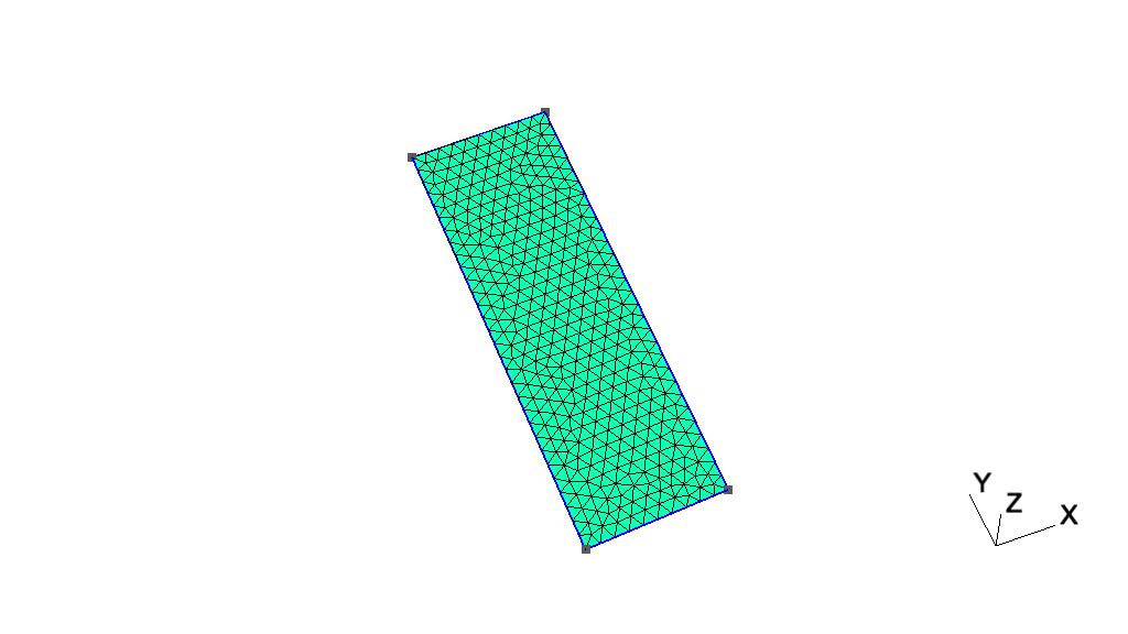
2.1 t1: Geometry basics, elementary entities, physical groups 
See t1.geo. Also available in C++ (t1.cpp), C (t1.c), Python (t1.py), Julia (t1.jl) and Fortran (t1.f90).
// -----------------------------------------------------------------------------
//
//  Gmsh GEO tutorial 1
//
//  Geometry basics, elementary entities, physical groups
//
// -----------------------------------------------------------------------------

// The simplest construction in Gmsh's scripting language is the
// `affectation'. The following command defines a new variable `lc':

lc = 1e-2;

// This variable can then be used in the definition of Gmsh's simplest
// `elementary entity', a `Point'. A Point is uniquely identified by a tag (a
// strictly positive integer; here `1') and defined by a list of four numbers:
// three coordinates (X, Y and Z) and the target mesh size (lc) close to the
// point:

Point(1) = {0, 0, 0, lc};

// The distribution of the mesh element sizes will then be obtained by
// interpolation of these mesh sizes throughout the geometry. Another method to
// specify mesh sizes is to use general mesh size Fields (see `t10.geo'). A
// particular case is the use of a background mesh (see `t7.geo').

// If no target mesh size of provided, a default uniform coarse size will be
// used for the model, based on the overall model size.

// We can then define some additional points. All points should have different
// tags:

Point(2) = {.1, 0,  0, lc};
Point(3) = {.1, .3, 0, lc};
Point(4) = {0,  .3, 0, lc};

// Curves are Gmsh's second type of elementary entities, and, amongst curves,
// straight lines are the simplest. A straight line is identified by a tag and
// is defined by a list of two point tags. In the commands below, for example,
// the line 1 starts at point 1 and ends at point 2.
//
// Note that curve tags are separate from point tags - hence we can reuse tag
// `1' for our first curve. And as a general rule, elementary entity tags in
// Gmsh have to be unique per geometrical dimension.

Line(1) = {1, 2};
Line(2) = {3, 2};
Line(3) = {3, 4};
Line(4) = {4, 1};

// The third elementary entity is the surface. In order to define a simple
// rectangular surface from the four curves defined above, a curve loop has
// first to be defined. A curve loop is also identified by a tag (unique amongst
// curve loops) and defined by an ordered list of connected curves, a sign being
// associated with each curve (depending on the orientation of the curve to form
// a loop):

Curve Loop(1) = {4, 1, -2, 3};

// We can then define the surface as a list of curve loops (only one here,
// representing the external contour, since there are no holes--see `t4.geo' for
// an example of a surface with a hole):

Plane Surface(1) = {1};

// At this level, Gmsh knows everything to display the rectangular surface 1 and
// to mesh it. An optional step is needed if we want to group elementary
// geometrical entities into more meaningful groups, e.g. to define some
// mathematical ("domain", "boundary"), functional ("left wing", "fuselage") or
// material ("steel", "carbon") properties.
//
// Such groups are called "Physical Groups" in Gmsh. By default, if physical
// groups are defined, Gmsh will export in output files only mesh elements that
// belong to at least one physical group. (To force Gmsh to save all elements,
// whether they belong to physical groups or not, set `Mesh.SaveAll=1;', or
// specify `-save_all' on the command line.) Physical groups are also identified
// by tags, i.e. strictly positive integers, that should be unique per dimension
// (0D, 1D, 2D or 3D). Physical groups can also be given names.
//
// Here we define a physical curve that groups the left, bottom and right curves
// in a single group (with prescribed tag 5); and a physical surface with name
// "My surface" (with an automatic tag) containing the geometrical surface 1:

Physical Curve(5) = {1, 2, 4};
Physical Surface("My surface") = {1};

// Now that the geometry is complete, you can
// - either open this file with Gmsh and select `2D' in the `Mesh' module to
//   create a mesh; then select `Save' to save it to disk in the default format
//   (or use `File->Export' to export in other formats);
// - or run `gmsh t1.geo -2` to mesh in batch mode on the command line.

// You could also uncomment the following lines in this script:
//
//   Mesh 2;
//   Save "t1.msh";
//
// which would lead Gmsh to mesh and save the mesh every time the file is
// parsed. (To simply parse the file from the command line, you can use `gmsh
// t1.geo -')

// By default, Gmsh saves meshes in the latest version of the Gmsh mesh file
// format (the `MSH' format). You can save meshes in other mesh formats by
// specifying a filename with a different extension in the GUI, on the command
// line or in scripts. For example
//
//   Save "t1.unv";
//
// will save the mesh in the UNV format. You can also save the mesh in older
// versions of the MSH format:
//
// - In the GUI: open `File->Export', enter your `filename.msh' and then pick
//   the version in the dropdown menu.
// - On the command line: use the `-format' option (e.g. `gmsh file.geo -format
//   msh2 -2').
// - In a `.geo' script: add `Mesh.MshFileVersion = x.y;' for any version
//   number `x.y'.
// - As an alternative method, you can also not specify the format explicitly,
//   and just choose a filename with the `.msh2' or `.msh4' extension.

// Note that starting with Gmsh 3.0, models can be built using other geometry
// kernels than the default built-in kernel. By specifying
//
//   SetFactory("OpenCASCADE");
//
// any subsequent command in the `.geo' file would be handled by the OpenCASCADE
// geometry kernel instead of the built-in kernel. Different geometry kernels
// have different features. With OpenCASCADE, instead of defining the surface by
// successively defining 4 points, 4 curves and 1 curve loop, one can define the
// rectangular surface directly with
//
//   Rectangle(2) = {.2, 0, 0, .1, .3};
//
// The underlying curves and points could be accessed with the `Boundary' or
// `CombinedBoundary' operators.
//
// See e.g. `t16.geo', `t18.geo', `t19.geo' or `t20.geo' for complete examples
// based on OpenCASCADE, and `examples/boolean' for more.
2.2 t2: Transformations, extruded geometries, volumes 
See t2.geo. Also available in C++ (t2.cpp), C (t2.c), Python (t2.py), Julia (t2.jl) and Fortran (t2.f90).
// -----------------------------------------------------------------------------
//
//  Gmsh GEO tutorial 2
//
//  Transformations, extruded geometries, volumes
//
// -----------------------------------------------------------------------------

// We first include the previous tutorial file, in order to use it as a basis
// for this one. Including a file is equivalent to copy-pasting its contents:

Include "t1.geo";

// We can then add new points and curves in the same way as we did in `t1.geo':

Point(5) = {0, .4, 0, lc};
Line(5) = {4, 5};

// Gmsh also provides tools to transform (translate, rotate, etc.)
// elementary entities or copies of elementary entities. For example, point
// 5 can be moved by 0.02 to the left with:

Translate {-0.02, 0, 0} { Point{5}; }

// And it can be further rotated by -Pi/4 around (0, 0.3, 0) (with the rotation
// along the z axis) with:

Rotate {{0,0,1}, {0,0.3,0}, -Pi/4} { Point{5}; }

// Note that there are no units in Gmsh: coordinates are just numbers - it's up
// to the user to associate a meaning to them.

// Point 3 can be duplicated and translated by 0.05 along the y axis:

Translate {0, 0.05, 0} { Duplicata{ Point{3}; } }

// This command created a new point with an automatically assigned tag. This tag
// can be obtained using the graphical user interface by hovering the mouse over
// the point: in this case, the new point has tag `6'.

Line(7) = {3, 6};
Line(8) = {6, 5};
Curve Loop(10) = {5,-8,-7,3};
Plane Surface(11) = {10};

// To automate the workflow, instead of using the graphical user interface to
// obtain the tags of newly created entities, one can use the return value of
// the transformation commands directly. For example, the `Translate' command
// returns a list containing the tags of the translated entities. Let's
// translate copies of the two surfaces 1 and 11 to the right with the following
// command:

my_new_surfs[] = Translate {0.12, 0, 0} { Duplicata{ Surface{1, 11}; } };

// my_new_surfs[] (note the square brackets, and the `;' at the end of the
// command) denotes a list, which contains the tags of the two new surfaces
// (check `Tools->Message console' to see the message):

Printf("New surfaces '%g' and '%g'", my_new_surfs[0], my_new_surfs[1]);

// In Gmsh lists use square brackets for their definition (mylist[] = {1, 2,
// 3};) as well as to access their elements (myotherlist[] = {mylist[0],
// mylist[2]}; mythirdlist[] = myotherlist[];), with list indexing starting at
// 0. To get the size of a list, use the hash (pound): len = #mylist[].
//
// Note that parentheses can also be used instead of square brackets, so that we
// could also write `myfourthlist() = {mylist(0), mylist(1)};'.

// Volumes are the fourth type of elementary entities in Gmsh. In the same way
// one defines curve loops to build surfaces, one has to define surface loops
// (i.e. `shells') to build volumes. The following volume does not have holes
// and thus consists of a single surface loop:

Point(100) = {0., 0.3, 0.12, lc};  Point(101) = {0.1, 0.3, 0.12, lc};
Point(102) = {0.1, 0.35, 0.12, lc};

xyz[] = Point{5}; // Get coordinates of point 5
Point(103) = {xyz[0], xyz[1], 0.12, lc};

Line(110) = {4, 100};   Line(111) = {3, 101};
Line(112) = {6, 102};   Line(113) = {5, 103};
Line(114) = {103, 100}; Line(115) = {100, 101};
Line(116) = {101, 102}; Line(117) = {102, 103};

Curve Loop(118) = {115, -111, 3, 110};  Plane Surface(119) = {118};
Curve Loop(120) = {111, 116, -112, -7}; Plane Surface(121) = {120};
Curve Loop(122) = {112, 117, -113, -8}; Plane Surface(123) = {122};
Curve Loop(124) = {114, -110, 5, 113};  Plane Surface(125) = {124};
Curve Loop(126) = {115, 116, 117, 114}; Plane Surface(127) = {126};

Surface Loop(128) = {127, 119, 121, 123, 125, 11};
Volume(129) = {128};

// When a volume can be extruded from a surface, it is usually easier to use the
// `Extrude' command directly instead of creating all the points, curves and
// surfaces by hand. For example, the following command extrudes the surface 11
// along the z axis and automatically creates a new volume (as well as all the
// needed points, curves and surfaces):

Extrude {0, 0, 0.12} { Surface{my_new_surfs[1]}; }

// The following command permits to manually assign a mesh size to some of the
// new points:

MeshSize {103, 105, 109, 102, 28, 24, 6, 5} = lc * 3;

// We finally group volumes 129 and 130 in a single physical group with tag `1'
// and name "The volume":

Physical Volume("The volume", 1) = {129,130};

// Note that, if the transformation tools are handy to create complex
// geometries, it is also sometimes useful to generate the `flat' geometry, with
// an explicit representation of all the elementary entities.
//
// This can be achieved with `File->Export' by selecting the `Gmsh Unrolled GEO'
// format, or by adding
//
//   Save "file.geo_unrolled";
//
// in the script. It can also be achieved with `gmsh t2.geo -0' on the command
// line.
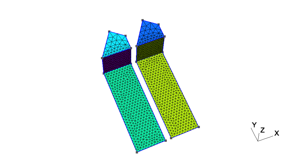
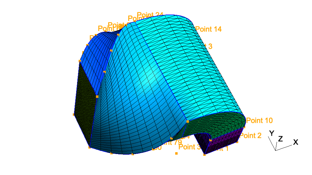
2.3 t3: Extruded meshes, ONELAB parameters, options 
See t3.geo. Also available in C++ (t3.cpp), Python (t3.py), Julia (t3.jl) and Fortran (t3.f90).
// -----------------------------------------------------------------------------
//
//  Gmsh GEO tutorial 3
//
//  Extruded meshes, ONELAB parameters, options
//
// -----------------------------------------------------------------------------

// Again, we start by including the first tutorial:

Include "t1.geo";

// As in `t2.geo', we plan to perform an extrusion along the z axis.  But here,
// instead of only extruding the geometry, we also want to extrude the 2D
// mesh. This is done with the same `Extrude' command, but by specifying element
// 'Layers' (2 layers in this case, the first one with 8 subdivisions and the
// second one with 2 subdivisions, both with a height of h/2):

h = 0.1;

Extrude {0,0,h} {
  Surface{1}; Layers{ {8,2}, {0.5,1} };
}

// The extrusion can also be performed with a rotation instead of a translation,
// and the resulting mesh can be recombined into prisms (we use only one layer
// here, with 7 subdivisions). All rotations are specified by an axis direction
// ({0,1,0}), an axis point ({-0.1,0,0.1}) and a rotation angle (-Pi/2):

Extrude { {0,1,0} , {-0.1,0,0.1} , -Pi/2 } {
  Surface{28}; Layers{7}; Recombine;
}

// Using the built-in geometry kernel, only rotations with angles < Pi are
// supported. To do a full turn, you will thus need to apply at least 3
// rotations. The OpenCASCADE geometry kernel does not have this limitation.

// Note that a translation ({-2*h,0,0}) and a rotation ({1,0,0}, {0,0.15,0.25},
// Pi/2) can also be combined to form a "twist". Here the angle is specified as
// a ONELAB parameter, using the `DefineConstant' syntax. ONELAB parameters can
// be modified interactively in the GUI, and can be exchanged with other codes
// connected to the same ONELAB database:

DefineConstant[ angle = {90, Min 0, Max 120, Step 1,
                         Name "Parameters/Twisting angle"} ];

// In more details, `DefineConstant' allows you to assign the value of the
// ONELAB parameter "Parameters/Twisting angle" to the variable `angle'. If the
// ONELAB parameter does not exist in the database, `DefineConstant' will create
// it and assign the default value `90'. Moreover, if the variable `angle' was
// defined before the call to `DefineConstant', the `DefineConstant' call would
// simply be skipped. This allows to build generic parametric models, whose
// parameters can be frozen from the outside - the parameters ceasing to be
// "parameters".
//
// An interesting use of this feature is in conjunction with the `-setnumber
// name value' command line switch, which defines a variable `name' with value
// `value'. Calling `gmsh t3.geo -setnumber angle 30' would define `angle'
// before the `DefineConstant', making `t3.geo' non-parametric
// ("Parameters/Twisting angle" will not be created in the ONELAB database and
// will not be available for modification in the graphical user interface).

out[] = Extrude { {-2*h,0,0}, {1,0,0} , {0,0.15,0.25} , angle * Pi / 180 } {
  Surface{50}; Layers{10}; Recombine;
};

// In this last extrusion command we retrieved the volume number
// programmatically by using the return value (a list) of the `Extrude'
// command. This list contains the "top" of the extruded surface (in `out[0]'),
// the newly created volume (in `out[1]') and the tags of the lateral surfaces
// (in `out[2]', `out[3]', ...).

// We can then define a new physical volume (with tag 101) to group all the
// elementary volumes:

Physical Volume(101) = {1, 2, out[1]};

// Let us now change some options... Since all interactive options are
// accessible in Gmsh's scripting language, we can for example make point tags
// visible or redefine some colors directly in the input file:

Geometry.PointNumbers = 1;
Geometry.Color.Points = Orange;
General.Color.Text = White;
Mesh.Color.Points = {255, 0, 0};

// Note that all colors can be defined literally or numerically, i.e.
// `Mesh.Color.Points = Red' is equivalent to `Mesh.Color.Points = {255,0,0}';
// and also note that, as with user-defined variables, the options can be used
// either as right or left hand sides, so that the following command will set
// the surface color to the same color as the points:

Geometry.Color.Surfaces = Geometry.Color.Points;

// You can use the `Help->Current Options and Workspace' menu to see the current
// values of all options. To save all the options in a file, use
// `File->Export->Gmsh Options'. To associate the current options with the
// current file use `File->Save Model Options'. To save the current options for
// all future Gmsh sessions use `File->Save Options As Default'.
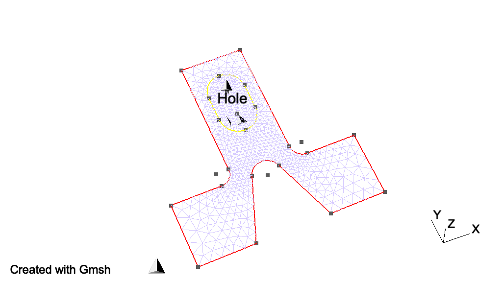
2.4 t4: Built-in functions, holes in surfaces, annotations, entity colors 
See t4.geo. Also available in C++ (t4.cpp), Python (t4.py), Julia (t4.jl) and Fortran (t4.f90).
// -----------------------------------------------------------------------------
//
//  Gmsh GEO tutorial 4
//
//  Built-in functions, holes in surfaces, annotations, entity colors
//
// -----------------------------------------------------------------------------

// As usual, we start by defining some variables:

cm = 1e-02;
e1 = 4.5 * cm; e2 = 6 * cm / 2; e3 =  5 * cm / 2;
h1 = 5 * cm; h2 = 10 * cm; h3 = 5 * cm; h4 = 2 * cm; h5 = 4.5 * cm;
R1 = 1 * cm; R2 = 1.5 * cm; r = 1 * cm;
Lc1 = 0.01;
Lc2 = 0.003;

// We can use all the usual mathematical functions (note the capitalized first
// letters), plus some useful functions like Hypot(a, b) := Sqrt(a^2 + b^2):

ccos = (-h5*R1 + e2 * Hypot(h5, Hypot(e2, R1))) / (h5^2 + e2^2);
ssin = Sqrt(1 - ccos^2);

// Then we define some points and some lines using these variables:

Point(1) = {-e1-e2, 0    , 0, Lc1}; Point(2) = {-e1-e2, h1   , 0, Lc1};
Point(3) = {-e3-r , h1   , 0, Lc2}; Point(4) = {-e3-r , h1+r , 0, Lc2};
Point(5) = {-e3   , h1+r , 0, Lc2}; Point(6) = {-e3   , h1+h2, 0, Lc1};
Point(7) = { e3   , h1+h2, 0, Lc1}; Point(8) = { e3   , h1+r , 0, Lc2};
Point(9) = { e3+r , h1+r , 0, Lc2}; Point(10)= { e3+r , h1   , 0, Lc2};
Point(11)= { e1+e2, h1   , 0, Lc1}; Point(12)= { e1+e2, 0    , 0, Lc1};
Point(13)= { e2   , 0    , 0, Lc1};

Point(14)= { R1 / ssin, h5+R1*ccos, 0, Lc2};
Point(15)= { 0        , h5        , 0, Lc2};
Point(16)= {-R1 / ssin, h5+R1*ccos, 0, Lc2};
Point(17)= {-e2       , 0.0       , 0, Lc1};

Point(18)= {-R2 , h1+h3   , 0, Lc2}; Point(19)= {-R2 , h1+h3+h4, 0, Lc2};
Point(20)= { 0  , h1+h3+h4, 0, Lc2}; Point(21)= { R2 , h1+h3+h4, 0, Lc2};
Point(22)= { R2 , h1+h3   , 0, Lc2}; Point(23)= { 0  , h1+h3   , 0, Lc2};

Point(24)= { 0, h1+h3+h4+R2, 0, Lc2}; Point(25)= { 0, h1+h3-R2,    0, Lc2};

Line(1)  = {1 , 17};
Line(2)  = {17, 16};

// Gmsh provides other curve primitives than straight lines: splines, B-splines,
// circle arcs, ellipse arcs, etc. Here we define a new circle arc, starting at
// point 14 and ending at point 16, with the circle's center being the point 15:

Circle(3) = {14,15,16};

// Note that, in Gmsh, circle arcs should always be smaller than Pi. The
// OpenCASCADE geometry kernel does not have this limitation.

// We can then define additional lines and circles, as well as a new surface:

Line(4)  = {14, 13}; Line(5)   = {13, 12};   Line(6)    = {12, 11};
Line(7)  = {11, 10}; Circle(8) = {8, 9, 10}; Line(9)    = {8, 7};
Line(10) = {7, 6};   Line(11)  = {6, 5};     Circle(12) = {3, 4, 5};
Line(13) = {3, 2};   Line(14)  = {2, 1};     Line(15)   = {18, 19};
Circle(16) = {21, 20, 24}; Circle(17) = {24, 20, 19};
Circle(18) = {18, 23, 25}; Circle(19) = {25, 23, 22};
Line(20) = {21,22};

Curve Loop(21) = {17, -15, 18, 19, -20, 16};
Plane Surface(22) = {21};

// But we still need to define the exterior surface. Since this surface has a
// hole, its definition now requires two curves loops:

Curve Loop(23) = {11, -12, 13, 14, 1, 2, -3, 4, 5, 6, 7, -8, 9, 10};
Plane Surface(24) = {23, 21};

// As a general rule, if a surface has N holes, it is defined by N+1 curve loops:
// the first loop defines the exterior boundary; the other loops define the
// boundaries of the holes.

// Finally, we can add some comments by embedding a post-processing view
// containing some strings:

View "comments" {
  // Add a text string in window coordinates, 10 pixels from the left and 10
  // pixels from the bottom, using the `StrCat' function to concatenate strings:
  T2(10, -10, 0){ StrCat("Created on ", Today, " with Gmsh") };

  // Add a text string in model coordinates centered at (X,Y,Z) = (0, 0.11, 0):
  T3(0, 0.11, 0, TextAttributes("Align", "Center", "Font", "Helvetica")){
    "Hole"
  };

  // If a string starts with `file://', the rest is interpreted as an image
  // file. For 3D annotations, the size in model coordinates can be specified
  // after a `@' symbol in the form `widthxheight' (if one of `width' or
  // `height' is zero, natural scaling is used; if both are zero, original image
  // dimensions in pixels are used):
  T3(0, 0.09, 0, TextAttributes("Align", "Center")){
    "file://t4_image.png@0.01x0"
  };

  // The 3D orientation of the image can be specified by proving the direction
  // of the bottom and left edge of the image in model space:
  T3(-0.01, 0.09, 0, 0){ "file://t4_image.png@0.01x0,0,0,1,0,1,0" };

  // The image can also be drawn in "billboard" mode, i.e. always parallel to
  // the camera, by using the `#' symbol:
  T3(0, 0.12, 0, TextAttributes("Align", "Center")){
    "file://t4_image.png@0.01x0#"
  };

  // The size of 2D annotations is given directly in pixels:
  T2(350, -7, 0){ "file://t4_image.png@20x0" };
};

// This post-processing view is in the "parsed" format, i.e. it is interpreted
// using the same parser as the `.geo' file. For large post-processing datasets,
// that contain actual field values defined on a mesh, you should use the MSH
// file format instead, which allows to efficiently store continuous or
// discontinuous scalar, vector and tensor fields, or arbitrary polynomial
// order.

// Views and geometrical entities can be made to respond to double-click events,
// here to print some messages to the console:

View[0].DoubleClickedCommand = "Printf('View[0] has been double-clicked!');";
Geometry.DoubleClickedCurveCommand = "Printf('Curve %g has been double-clicked!',
  Geometry.DoubleClickedEntityTag);";

// We can also change the color of some entities:

Color Grey50{ Surface{ 22 }; }
Color Purple{ Surface{ 24 }; }
Color Red{ Curve{ 1:14 }; }
Color Yellow{ Curve{ 15:20 }; }
2.5 t5: Mesh sizes, macros, loops, holes in volumes 
See t5.geo. Also available in C++ (t5.cpp), Python (t5.py), Julia (t5.jl) and Fortran (t5.f90).
// -----------------------------------------------------------------------------
//
//  Gmsh GEO tutorial 5
//
//  Mesh sizes, macros, loops, holes in volumes
//
// -----------------------------------------------------------------------------

// We start by defining some target mesh sizes:

lcar1 = .1;
lcar2 = .0005;
lcar3 = .055;

// If we wanted to change these mesh sizes globally (without changing the above
// definitions), we could give a global scaling factor for all mesh sizes on the
// command line with the `-clscale' option (or with `Mesh.MeshSizeFactor' in an
// option file). For example, with:
//
// > gmsh t5.geo -clscale 1
//
// this input file produces a mesh of approximately 3000 nodes and 14,000
// tetrahedra. With
//
// > gmsh t5.geo -clscale 0.2
//
// the mesh counts approximately 231,000 nodes and 1,360,000 tetrahedra. You can
// check mesh statistics in the graphical user interface with the
// `Tools->Statistics' menu.
//
// See `t10.geo' for more information about mesh sizes.

// We proceed by defining some elementary entities describing a truncated cube:

Point(1) = {0.5,0.5,0.5,lcar2}; Point(2) = {0.5,0.5,0,lcar1};
Point(3) = {0,0.5,0.5,lcar1};   Point(4) = {0,0,0.5,lcar1};
Point(5) = {0.5,0,0.5,lcar1};   Point(6) = {0.5,0,0,lcar1};
Point(7) = {0,0.5,0,lcar1};     Point(8) = {0,1,0,lcar1};
Point(9) = {1,1,0,lcar1};       Point(10) = {0,0,1,lcar1};
Point(11) = {0,1,1,lcar1};      Point(12) = {1,1,1,lcar1};
Point(13) = {1,0,1,lcar1};      Point(14) = {1,0,0,lcar1};

Line(1) = {8,9};    Line(2) = {9,12};  Line(3) = {12,11};
Line(4) = {11,8};   Line(5) = {9,14};  Line(6) = {14,13};
Line(7) = {13,12};  Line(8) = {11,10}; Line(9) = {10,13};
Line(10) = {10,4};  Line(11) = {4,5};  Line(12) = {5,6};
Line(13) = {6,2};   Line(14) = {2,1};  Line(15) = {1,3};
Line(16) = {3,7};   Line(17) = {7,2};  Line(18) = {3,4};
Line(19) = {5,1};   Line(20) = {7,8};  Line(21) = {6,14};

Curve Loop(22) = {-11,-19,-15,-18};   Plane Surface(23) = {22};
Curve Loop(24) = {16,17,14,15};       Plane Surface(25) = {24};
Curve Loop(26) = {-17,20,1,5,-21,13}; Plane Surface(27) = {26};
Curve Loop(28) = {-4,-1,-2,-3};       Plane Surface(29) = {28};
Curve Loop(30) = {-7,2,-5,-6};        Plane Surface(31) = {30};
Curve Loop(32) = {6,-9,10,11,12,21};  Plane Surface(33) = {32};
Curve Loop(34) = {7,3,8,9};           Plane Surface(35) = {34};
Curve Loop(36) = {-10,18,-16,-20,4,-8}; Plane Surface(37) = {36};
Curve Loop(38) = {-14,-13,-12,19};    Plane Surface(39) = {38};

// Instead of using included files, we now use a user-defined macro in order
// to carve some holes in the cube:

Macro CheeseHole

  // In the following commands we use the reserved variable name `newp', which
  // automatically selects a new point tag. Analogously to `newp', the special
  // variables `newc', `newcl, `news', `newsl' and `newv' select new curve,
  // curve loop, surface, surface loop and volume tags.
  //
  // If `Geometry.OldNewReg' is set to 0, the new tags are chosen as the highest
  // current tag for each category (points, curves, curve loops, ...), plus
  // one. By default, for backward compatibility, `Geometry.OldNewReg' is set
  // to 1, and only two categories are used: one for points and one for the
  // rest.

  p1 = newp; Point(p1) = {x,  y,  z,  lcar3};
  p2 = newp; Point(p2) = {x+r,y,  z,  lcar3};
  p3 = newp; Point(p3) = {x,  y+r,z,  lcar3};
  p4 = newp; Point(p4) = {x,  y,  z+r,lcar3};
  p5 = newp; Point(p5) = {x-r,y,  z,  lcar3};
  p6 = newp; Point(p6) = {x,  y-r,z,  lcar3};
  p7 = newp; Point(p7) = {x,  y,  z-r,lcar3};

  c1 = newc; Circle(c1) = {p2,p1,p7}; c2 = newc; Circle(c2) = {p7,p1,p5};
  c3 = newc; Circle(c3) = {p5,p1,p4}; c4 = newc; Circle(c4) = {p4,p1,p2};
  c5 = newc; Circle(c5) = {p2,p1,p3}; c6 = newc; Circle(c6) = {p3,p1,p5};
  c7 = newc; Circle(c7) = {p5,p1,p6}; c8 = newc; Circle(c8) = {p6,p1,p2};
  c9 = newc; Circle(c9) = {p7,p1,p3}; c10 = newc; Circle(c10) = {p3,p1,p4};
  c11 = newc; Circle(c11) = {p4,p1,p6}; c12 = newc; Circle(c12) = {p6,p1,p7};

  // We need non-plane surfaces to define the spherical holes. Here we use
  // `Surface', which can be used for surfaces with 3 or 4 curves on their
  // boundary. With the built-in kernel, if all the curves are circle arcs with
  // the same center, a spherical patch is created; otherwise transfinite
  // interpolation is used. With the OpenCASCADE kernel, `Surface' can be used
  // with an arbitrary number of boundary curves, and will fit a BSpline patch
  // through them.

  l1 = newcl; Curve Loop(l1) = {c5,c10,c4};
  l2 = newcl; Curve Loop(l2) = {c9,-c5,c1};
  l3 = newcl; Curve Loop(l3) = {c12,-c8,-c1};
  l4 = newcl; Curve Loop(l4) = {c8,-c4,c11};
  l5 = newcl; Curve Loop(l5) = {-c10,c6,c3};
  l6 = newcl; Curve Loop(l6) = {-c11,-c3,c7};
  l7 = newcl; Curve Loop(l7) = {-c2,-c7,-c12};
  l8 = newcl; Curve Loop(l8) = {-c6,-c9,c2};

  s1 = news; Surface(s1) = {l1};
  s2 = news; Surface(s2) = {l2};
  s3 = news; Surface(s3) = {l3};
  s4 = news; Surface(s4) = {l4};
  s5 = news; Surface(s5) = {l5};
  s6 = news; Surface(s6) = {l6};
  s7 = news; Surface(s7) = {l7};
  s8 = news; Surface(s8) = {l8};

  // We then store the surface loops tags in a list for later reference (we will
  // need these to define the final volume):

  theloops[t] = newsl;
  Surface Loop(theloops[t]) = {s1, s2, s3, s4, s5, s6, s7, s8};

  thehole = newv;
  Volume(thehole) = theloops[t];

Return

// We can use a `For' loop to generate five holes in the cube:

x = 0; y = 0.75; z = 0; r = 0.09;

For t In {1:5}

  x += 0.166;
  z += 0.166;

  // We call the `CheeseHole' macro:

  Call CheeseHole;

  // We define a physical volume for each hole:

  Physical Volume (t) = thehole;

  // We also print some variables on the terminal (note that, since all
  // variables in `.geo' files are treated internally as floating point numbers,
  // the format string should only contain valid floating point format
  // specifiers like `%g', `%f', '%e', etc.):

  Printf("Hole %g (center = {%g,%g,%g}, radius = %g) has number %g!",
	 t, x, y, z, r, thehole);

EndFor

// We can then define the surface loop for the exterior surface of the cube:

theloops[0] = newreg;
Surface Loop(theloops[0]) = {23:39:2};

// The volume of the cube, without the 5 holes, is now defined by 6 surface
// loops: the first surface loop defines the exterior surface; the surface loops
// other than the first one define holes.  (Again, to reference an array of
// variables, its identifier is followed by square brackets):

Volume(186) = {theloops[]};

// Note that using solid modelling with the OpenCASCADE geometry kernel, the
// same geometry could be built quite differently: see `t16.geo'.

// We finally define a physical volume for the elements discretizing the cube,
// without the holes (for which physical groups were already created in the
// `For' loop):

Physical Volume (10) = 186;

// We could make only part of the model visible to only mesh this subset:
//
// Hide {:}
// Recursive Show { Volume{129}; }
// Mesh.MeshOnlyVisible=1;

// Meshing algorithms can changed globally using options:

Mesh.Algorithm = 6; // Frontal-Delaunay for 2D meshes

// They can also be set for individual surfaces, e.g.

MeshAlgorithm Surface {31, 35} = 1; // MeshAdapt on surfaces 31 and 35

// To generate a curvilinear mesh and optimize it to produce provably valid
// curved elements (see A. Johnen, J.-F. Remacle and C. Geuzaine. Geometric
// validity of curvilinear finite elements. Journal of Computational Physics
// 233, pp. 359-372, 2013; and T. Toulorge, C. Geuzaine, J.-F. Remacle,
// J. Lambrechts. Robust untangling of curvilinear meshes. Journal of
// Computational Physics 254, pp. 8-26, 2013), you can uncomment the following
// lines:
//
// Mesh.ElementOrder = 2;
// Mesh.HighOrderOptimize = 2;
2.6 t6: Transfinite meshes, deleting entities 
See t6.geo. Also available in C++ (t6.cpp), C (t6.c), Python (t6.py), Julia (t6.jl) and Fortran (t6.f90).
// -----------------------------------------------------------------------------
//
//  Gmsh GEO tutorial 6
//
//  Transfinite meshes, deleting entities
//
// -----------------------------------------------------------------------------

// Let's use the geometry from the first tutorial as a basis for this one:
lc = 1e-2;
Point(1) = {0, 0, 0, lc};
Point(2) = {.1, 0,  0, lc};
Point(3) = {.1, .3, 0, lc};
Point(4) = {0,  .3, 0, lc};
Line(1) = {1, 2};
Line(2) = {3, 2};
Line(3) = {3, 4};
Line(4) = {4, 1};
Curve Loop(1) = {4, 1, -2, 3};
Plane Surface(1) = {1};

// Delete the surface and the left line, and replace the line with 3 new ones:
Delete{ Surface{1}; Curve{4}; }

p1 = newp; Point(p1) = {-0.05, 0.05, 0, lc};
p2 = newp; Point(p2) = {-0.05, 0.1, 0, lc};

l1 = newc; Line(l1) = {1, p1};
l2 = newc; Line(l2) = {p1, p2};
l3 = newc; Line(l3) = {p2, 4};

// Create a surface:
Curve Loop(2) = {2, -1, l1, l2, l3, -3};
Plane Surface(1) = {-2};

// The `Transfinite Curve' meshing constraints explicitly specifies the location
// of the nodes on the curve. For example, the following command forces 20
// uniformly placed nodes on curve 2 (including the nodes on the two end
// points):
Transfinite Curve{2} = 20;

// Let's put 20 points total on combination of curves `l1', `l2' and `l3'
// (beware that the points `p1' and `p2' are shared by the curves, so we do not
// create 6 + 6 + 10 = 22 nodes, but 20!)
Transfinite Curve{l1} = 6;
Transfinite Curve{l2} = 6;
Transfinite Curve{l3} = 10;

// Finally, we put 30 nodes following a geometric progression on curve 1
// (reversed) and on curve 3:
Transfinite Curve{-1, 3} = 30 Using Progression 1.2;

// The `Transfinite Surface' meshing constraint uses a transfinite interpolation
// algorithm in the parametric plane of the surface to connect the nodes on the
// boundary using a structured grid. If the surface has more than 4 corner
// points, the corners of the transfinite interpolation have to be specified by
// hand:
Transfinite Surface{1} = {1, 2, 3, 4};

// To create quadrangles instead of triangles, one can use the `Recombine'
// command:
Recombine Surface{1};

// When the surface has only 3 or 4 points on its boundary the list of corners
// can be omitted in the `Transfinite Surface' constraint:
Point(7) = {0.2, 0.2, 0, 1.0};
Point(8) = {0.2, 0.1, 0, 1.0};
Point(9) = {0.25, 0.2, 0, 1.0};
Point(10) = {0.3, 0.1, 0, 1.0};
Line(10) = {8, 10};
Line(11) = {10, 9};
Line(12) = {9, 7};
Line(13) = {7, 8};
Curve Loop(14) = {10, 11, 12, 13};
Plane Surface(15) = {14};
Transfinite Curve {10, 11, 12, 13} = 10;
Transfinite Surface{15};

// The way triangles are generated can be controlled by appending "Left",
// "Right" or "Alternate" after the `Transfinite Surface' command. Try e.g.
//
// Transfinite Surface{15} Alternate;

// Finally we apply an elliptic smoother to the grid to have a more regular
// mesh:
Mesh.Smoothing = 100;
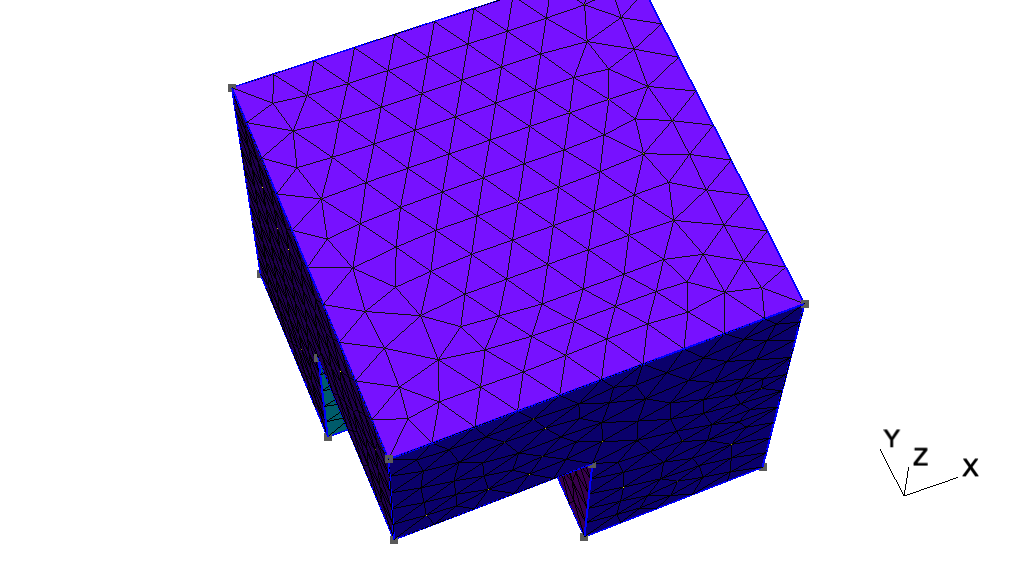
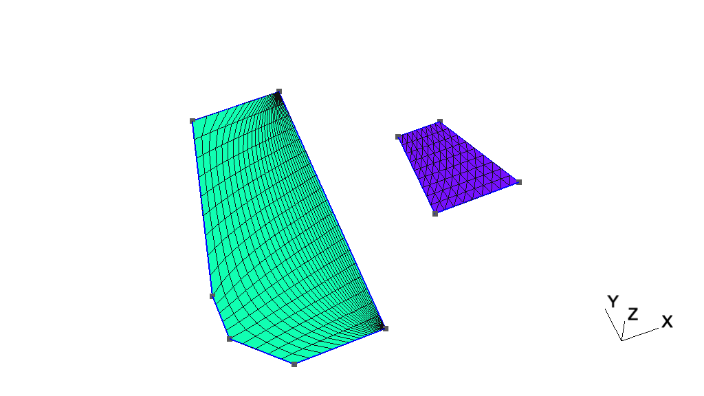
2.7 t7: Background meshes 
See t7.geo. Also available in C++ (t7.cpp), Python (t7.py), Julia (t7.jl) and Fortran (t7.f90).
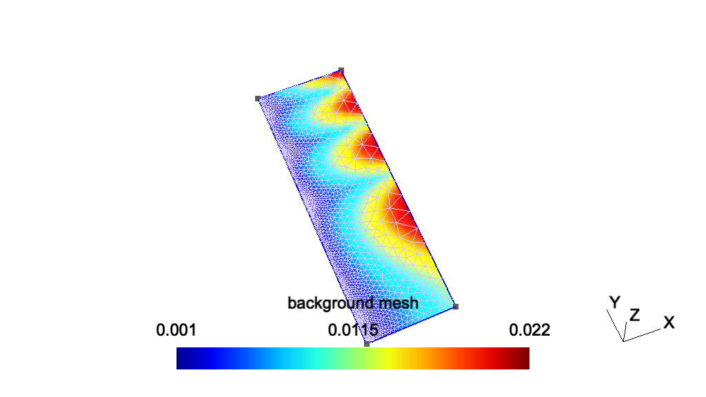
// -----------------------------------------------------------------------------
//
//  Gmsh GEO tutorial 7
//
//  Background meshes
//
// -----------------------------------------------------------------------------

// Mesh sizes can be specified very accurately by providing a background mesh,
// i.e., a post-processing view that contains the target mesh sizes.

// Merge a list-based post-processing view containing the target mesh sizes:
Merge "t7_bgmesh.pos";

// If the post-processing view was model-based instead of list-based (i.e. if it
// was based on an actual mesh), we would need to create a new model to contain
// the geometry so that meshing it does not destroy the background mesh. It's
// not necessary here since the view is list-based, but it does no harm:
NewModel;

// Merge the first tutorial geometry:
Merge "t1.geo";

// Apply the view as the current background mesh size field:
Background Mesh View[0];

// In order to compute the mesh sizes from the background mesh only, and
// disregard any other size constraints, one can set:
Mesh.MeshSizeExtendFromBoundary = 0;
Mesh.MeshSizeFromPoints = 0;
Mesh.MeshSizeFromCurvature = 0;

// See `t10.geo' for additional information: background meshes are actually a
// particular case of general "mesh size fields".
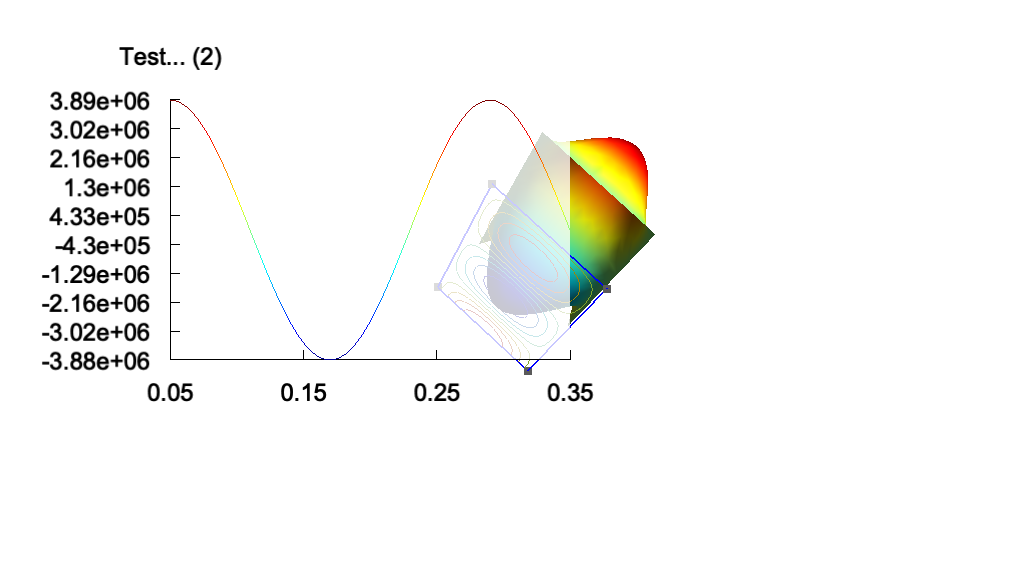
2.8 t8: Post-processing, image export and animations 
See t8.geo. Also available in C++ (t8.cpp), Python (t8.py), Julia (t8.jl) and Fortran (t8.f90).
// -----------------------------------------------------------------------------
//
//  Gmsh GEO tutorial 8
//
//  Post-processing, image export and animations
//
// -----------------------------------------------------------------------------

// In addition to creating geometries and meshes, GEO scripts can also be used
// to manipulate post-processing datasets (called "views" in Gmsh).

// We first include `t1.geo' as well as some post-processing views:

Include "t1.geo";
Include "view1.pos";
Include "view1.pos";
Include "view4.pos";

// Gmsh can read post-processing views in various formats. Here the `view1.pos'
// and `view4.pos' files are in the Gmsh "parsed" format, which is interpreted
// directly by the GEO script parser. The parsed format should only be used for
// relatively small datasets of course: for larger datasets using e.g. MSH files
// is much more efficient.

// We then set some general options:

General.Trackball = 0;
General.RotationX = 0; General.RotationY = 0; General.RotationZ = 0;
General.Color.Background = White; General.Color.Foreground = Black;
General.Color.Text = Black;
General.Orthographic = 0;
General.Axes = 0; General.SmallAxes = 0;

// We also set some options for each post-processing view:

v0 = PostProcessing.NbViews-4;
v1 = v0+1; v2 = v0+2; v3 = v0+3;

View[v0].IntervalsType = 2;
View[v0].OffsetZ = 0.05;
View[v0].RaiseZ = 0;
View[v0].Light = 1;
View[v0].ShowScale = 0;
View[v0].SmoothNormals = 1;

View[v1].IntervalsType = 1;
View[v1].ColorTable = { Green, Blue };
View[v1].NbIso = 10;
View[v1].ShowScale = 0;

View[v2].Name = "Test...";
View[v2].Axes = 1;
View[v2].Color.Axes = Black;
View[v2].IntervalsType = 2;
View[v2].Type = 2;
View[v2].AutoPosition = 0;
View[v2].PositionX = 85;
View[v2].PositionY = 50;
View[v2].Width = 200;
View[v2].Height = 130;

View[v3].Visible = 0;

// You can save an MPEG movie directly by selecting `File->Export' in the
// GUI. Several predefined animations are setup, for looping on all the time
// steps in views, or for looping between views.

// But a script can be used to build much more complex animations, by changing
// options at run-time and re-rendering the graphics. Each frame can then be
// saved to disk as an image, and multiple frames can be encoded to form a
// movie. Below is an example of such a custom animation.

t = 0; // Initial step

// Loop on num from 1 to 3
For num In {1:3}

  View[v0].TimeStep = t; // Set time step
  View[v1].TimeStep = t;
  View[v2].TimeStep = t;
  View[v3].TimeStep = t;

  t = (View[v0].TimeStep < View[v0].NbTimeStep-1) ? t+1 : 0; // Increment

  View[v0].RaiseZ += 0.01/View[v0].Max * t; // Raise view v0

  If (num == 3)
    // Resize the graphics when num == 3, to create 640x480 frames
    General.GraphicsWidth = General.MenuWidth + 640;
    General.GraphicsHeight = 480;
  EndIf

  frames = 50;

  // Loop on num2 from 1 to frames
  For num2 In {1:frames}

    // Incrementally rotate the scene
    General.RotationX += 10;
    General.RotationY = General.RotationX / 3;
    General.RotationZ += 0.1;

    // Sleep for 0.01 second
    Sleep 0.01;

    // Draw the scene (one could use `DrawForceChanged' instead to force the
    // reconstruction of the vertex arrays, e.g. if changing element clipping)
    Draw;

    If (num == 3)
      // Uncomment the following lines to save each frame to an image file (the
      // `Print' command saves the graphical window; the `Sprintf' function
      // permits to create the file names on the fly):

      // Print Sprintf("t8-%g.gif", num2);
      // Print Sprintf("t8-%g.ppm", num2);
      // Print Sprintf("t8-%g.jpg", num2);
    EndIf

  EndFor

  If(num == 3)
    // Here we could make a system call to generate a movie. For example, with
    // ffmpeg:

    // System "ffmpeg -i t8-%d.jpg t8.mpg"
  EndIf

EndFor
2.9 t9: Plugins 
See t9.geo. Also available in C++ (t9.cpp), Python (t9.py), Julia (t9.jl) and Fortran (t9.f90).
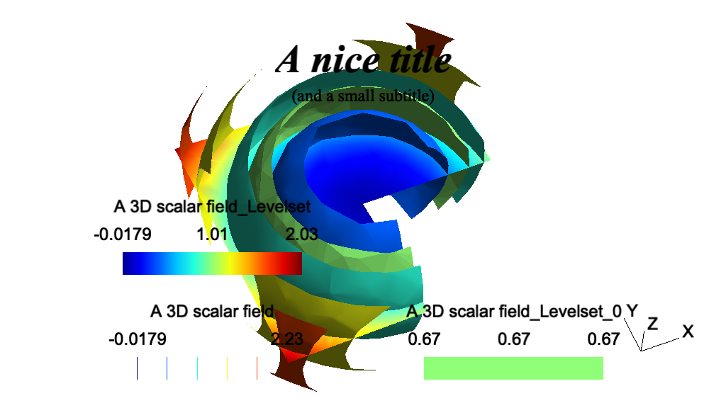
// -----------------------------------------------------------------------------
//
//  Gmsh GEO tutorial 9
//
//  Plugins
//
// -----------------------------------------------------------------------------

// Plugins can be added to Gmsh in order to extend its capabilities. For
// example, post-processing plugins can modify views, or create new views based
// on previously loaded views. Several default plugins are statically linked
// with Gmsh, e.g. Isosurface, CutPlane, CutSphere, Skin, Transform or Smooth.
//
// Plugins can be controlled in the same way as other options: either from the
// graphical interface (right click on the view button, then `Plugins'), or from
// the command file.

// Let us for example include a three-dimensional scalar view:

Include "view3.pos" ;

// We then set some options for the `Isosurface' plugin (which extracts an
// isosurface from a 3D scalar view), and run it:

Plugin(Isosurface).Value = 0.67 ; // Iso-value level
Plugin(Isosurface).View = 0 ; // Source view is View[0]
Plugin(Isosurface).Run ; // Run the plugin!

// We also set some options for the `CutPlane' plugin (which computes a section
// of a 3D view using the plane A*x+B*y+C*z+D=0), and then run it:

Plugin(CutPlane).A = 0 ;
Plugin(CutPlane).B = 0.2 ;
Plugin(CutPlane).C = 1 ;
Plugin(CutPlane).D = 0 ;
Plugin(CutPlane).View = 0 ;
Plugin(CutPlane).Run ;

// Add a title (By convention, for window coordinates a value greater than 99999
// represents the center. We could also use `General.GraphicsWidth / 2', but
// that would only center the string for the current window size.):

Plugin(Annotate).Text = "A nice title" ;
Plugin(Annotate).X = 1.e5;
Plugin(Annotate).Y = 50 ;
Plugin(Annotate).Font = "Times-BoldItalic" ;
Plugin(Annotate).FontSize = 28 ;
Plugin(Annotate).Align = "Center" ;
Plugin(Annotate).View = 0 ;
Plugin(Annotate).Run ;

Plugin(Annotate).Text = "(and a small subtitle)" ;
Plugin(Annotate).Y = 70 ;
Plugin(Annotate).Font = "Times-Roman" ;
Plugin(Annotate).FontSize = 12 ;
Plugin(Annotate).Run ;

// We finish by setting some options:

View[0].Light = 1;
View[0].IntervalsType = 1;
View[0].NbIso = 6;
View[0].SmoothNormals = 1;
View[1].IntervalsType = 2;
View[2].IntervalsType = 2;
2.10 t10: Mesh size fields 
See t10.geo. Also available in C++ (t10.cpp), Python (t10.py), Julia (t10.jl) and Fortran (t10.f90).
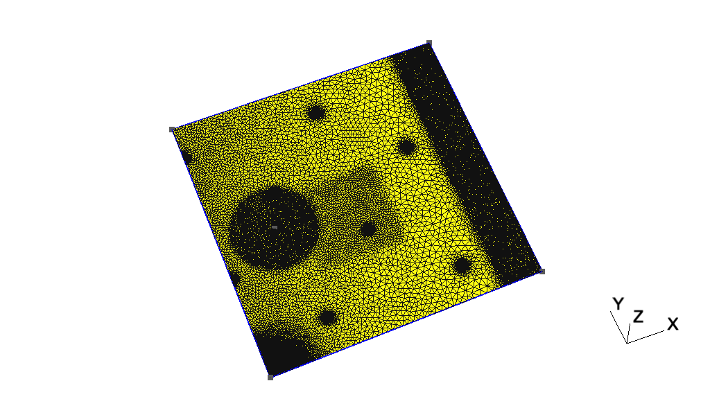
// -----------------------------------------------------------------------------
//
//  Gmsh GEO tutorial 10
//
//  Mesh size fields
//
// -----------------------------------------------------------------------------

// In addition to specifying target mesh sizes at the points of the geometry
// (see `t1.geo') or using a background mesh (see `t7.geo'), you can use general
// mesh size "Fields".

// Let's create a simple rectangular geometry
lc = .15;
Point(1) = {0.0,0.0,0,lc}; Point(2) = {1,0.0,0,lc};
Point(3) = {1,1,0,lc};     Point(4) = {0,1,0,lc};
Point(5) = {0.2,.5,0,lc};

Line(1) = {1,2}; Line(2) = {2,3}; Line(3) = {3,4}; Line(4) = {4,1};

Curve Loop(5) = {1,2,3,4}; Plane Surface(6) = {5};

// Say we would like to obtain mesh elements with size lc/30 near curve 2 and
// point 5, and size lc elsewhere. To achieve this, we can use two fields:
// "Distance", and "Threshold". We first define a Distance field (`Field[1]') on
// points 5 and on curve 2. This field returns the distance to point 5 and to
// (100 equidistant points on) curve 2.
Field[1] = Distance;
Field[1].PointsList = {5};
Field[1].CurvesList = {2};
Field[1].Sampling = 100;


// We then define a `Threshold' field, which uses the return value of the
// `Distance' field 1 in order to define a simple change in element size
// depending on the computed distances
//
// SizeMax -                     /------------------
//                              /
//                             /
//                            /
// SizeMin -o----------------/
//          |                |    |
//        Point         DistMin  DistMax
Field[2] = Threshold;
Field[2].InField = 1;
Field[2].SizeMin = lc / 30;
Field[2].SizeMax = lc;
Field[2].DistMin = 0.15;
Field[2].DistMax = 0.5;

// Say we want to modulate the mesh element sizes using a mathematical function
// of the spatial coordinates. We can do this with the MathEval field:
Field[3] = MathEval;
Field[3].F = "cos(4*3.14*x) * sin(4*3.14*y) / 10 + 0.101";

// We could also combine MathEval with values coming from other fields. For
// example, let's define a `Distance' field around point 1
Field[4] = Distance;
Field[4].PointsList = {1};

// We can then create a `MathEval' field with a function that depends on the
// return value of the `Distance' field 4, i.e., depending on the distance to
// point 1 (here using a cubic law, with minimum element size = lc / 100)
Field[5] = MathEval;
Field[5].F = Sprintf("F4^3 + %g", lc / 100);

// We could also use a `Box' field to impose a step change in element sizes
// inside a box
Field[6] = Box;
Field[6].VIn = lc / 15;
Field[6].VOut = lc;
Field[6].XMin = 0.3;
Field[6].XMax = 0.6;
Field[6].YMin = 0.3;
Field[6].YMax = 0.6;
Field[6].Thickness = 0.3;

// Many other types of fields are available: see the reference manual for a
// complete list. You can also create fields directly in the graphical user
// interface by selecting `Define->Size fields' in the `Mesh' module.

// Let's use the minimum of all the fields as the background mesh size field
Field[7] = Min;
Field[7].FieldsList = {2, 3, 5, 6};
Background Field = 7;

// To determine the size of mesh elements, Gmsh locally computes the minimum of
//
// 1) the size of the model bounding box;
// 2) if `Mesh.MeshSizeFromPoints' is set, the mesh size specified at
//    geometrical points;
// 3) if `Mesh.MeshSizeFromCurvature' is positive, the mesh size based on
//    curvature (the value specifying the number of elements per 2 * pi rad);
// 4) the background mesh size field;
// 5) any per-entity mesh size constraint.
//
// This value is then constrained in the interval [`Mesh.MeshSizeMin',
// `Mesh.MeshSizeMax'] and multiplied by `Mesh.MeshSizeFactor'. In addition,
// boundary mesh sizes are interpolated inside surfaces and/or volumes depending
// on the value of `Mesh.MeshSizeExtendFromBoundary' (which is set by default).
//
// When the element size is fully specified by a mesh size field (as it is in
// this example), it is thus often desirable to set

Mesh.MeshSizeExtendFromBoundary = 0;
Mesh.MeshSizeFromPoints = 0;
Mesh.MeshSizeFromCurvature = 0;

// This will prevent over-refinement due to small mesh sizes on the boundary.

// Finally, while the default "Frontal-Delaunay" 2D meshing algorithm
// (Mesh.Algorithm = 6) usually leads to the highest quality meshes, the
// "Delaunay" algorithm (Mesh.Algorithm = 5) will handle complex mesh size
// fields better - in particular size fields with large element size gradients:

Mesh.Algorithm = 5;
2.11 t11: Unstructured quadrangular meshes 
See t11.geo. Also available in C++ (t11.cpp), Python (t11.py), Julia (t11.jl) and Fortran (t11.f90).
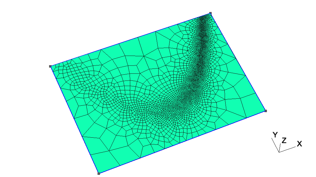
// -----------------------------------------------------------------------------
//
//  Gmsh GEO tutorial 11
//
//  Unstructured quadrangular meshes
//
// -----------------------------------------------------------------------------

// We have seen in tutorials `t3.geo' and `t6.geo' that extruded and transfinite
// meshes can be "recombined" into quads, prisms or hexahedra by using the
// "Recombine" keyword. Unstructured meshes can be recombined in the same
// way. Let's define a simple geometry with an analytical mesh size field:

Point(1) = {-1.25, -.5, 0}; Point(2) = {1.25, -.5, 0};
Point(3) = {1.25, 1.25, 0};  Point(4) = {-1.25, 1.25, 0};

Line(1) = {1, 2}; Line(2) = {2, 3};
Line(3) = {3, 4}; Line(4) = {4, 1};

Curve Loop(4) = {1, 2, 3, 4}; Plane Surface(100) = {4};

Field[1] = MathEval;
Field[1].F = "0.01*(1.0+30.*(y-x*x)*(y-x*x) + (1-x)*(1-x))";
Background Field = 1;

// To generate quadrangles instead of triangles, we can simply add

Recombine Surface{100};

// If we'd had several surfaces, we could have used `Recombine Surface {:};'.
// Yet another way would be to specify the global option "Mesh.RecombineAll =
// 1;".

// The default recombination algorithm is called "Blossom": it uses a minimum
// cost perfect matching algorithm to generate fully quadrilateral meshes from
// triangulations. More details about the algorithm can be found in the
// following paper: J.-F. Remacle, J. Lambrechts, B. Seny, E. Marchandise,
// A. Johnen and C. Geuzaine, "Blossom-Quad: a non-uniform quadrilateral mesh
// generator using a minimum cost perfect matching algorithm", International
// Journal for Numerical Methods in Engineering 89, pp. 1102-1119, 2012.

// For even better 2D (planar) quadrilateral meshes, you can try the
// experimental "Frontal-Delaunay for quads" meshing algorithm, which is a
// triangulation algorithm that enables to create right triangles almost
// everywhere: J.-F. Remacle, F. Henrotte, T. Carrier-Baudouin, E. Bechet,
// E. Marchandise, C. Geuzaine and T. Mouton. A frontal Delaunay quad mesh
// generator using the L^inf norm. International Journal for Numerical Methods
// in Engineering, 94, pp. 494-512, 2013. Uncomment the following line to try
// the Frontal-Delaunay algorithms for quads:
//
// Mesh.Algorithm = 8;

// The default recombination algorithm might leave some triangles in the mesh,
// if recombining all the triangles leads to badly shaped quads. In such cases,
// to generate full-quad meshes, you can either subdivide the resulting hybrid
// mesh (with Mesh.SubdivisionAlgorithm = 1), or use the full-quad recombination
// algorithm, which will automatically perform a coarser mesh followed by
// recombination, smoothing and subdivision. Uncomment the following line to try
// the full-quad algorithm:
//
// Mesh.RecombinationAlgorithm = 2; // or 3

// Note that you could also apply the recombination algorithm and/or the
// subdivision step explicitly after meshing, as follows:
//
// Mesh 2;
// RecombineMesh;
// Mesh.SubdivisionAlgorithm = 1;
// RefineMesh;
2.12 t12: Cross-patch meshing with compounds 
See t12.geo/ Also available in C++ (t12.cpp), Python (t12.py), Julia (t12.jl) and Fortran (t12.f90).
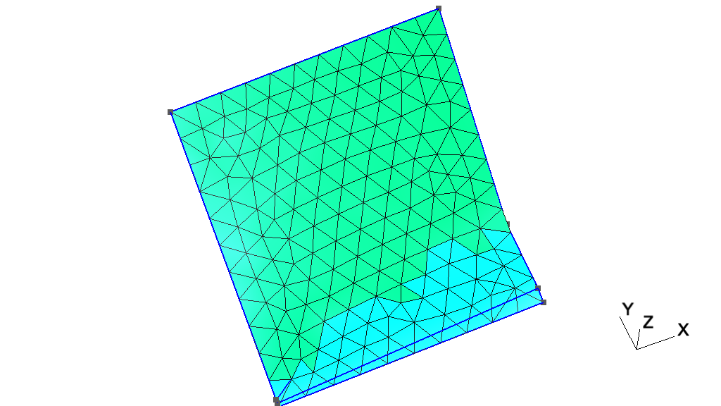
// -----------------------------------------------------------------------------
//
//  Gmsh GEO tutorial 12
//
//  Cross-patch meshing with compounds
//
// -----------------------------------------------------------------------------

// "Compound" meshing constraints allow to generate meshes across surface
// boundaries, which can be useful e.g. for imported CAD models (e.g. STEP) with
// undesired small features.

// When a `Compound Curve' or `Compound Surface' meshing constraint is given,
// at mesh generation time Gmsh
//  1. meshes the underlying elementary geometrical entities, individually
//  2. creates a discrete entity that combines all the individual meshes
//  3. computes a discrete parametrization (i.e. a piece-wise linear mapping)
//     on this discrete entity
//  4. meshes the discrete entity using this discrete parametrization instead
//     of the underlying geometrical description of the underlying elementary
//     entities making up the compound
//  5. optionally, reclassifies the mesh elements and nodes on the original
//     entities

// Step 3. above can only be performed if the mesh resulting from the
// combination of the individual meshes can be reparametrized, i.e. if the shape
// is "simple enough". If the shape is not amenable to reparametrization, you
// should create a full mesh of the geometry and first re-classify it to
// generate patches amenable to reparametrization (see `t13.geo').

// The mesh of the individual entities performed in Step 1. should usually be
// finer than the desired final mesh; this can be controlled with the
// `Mesh.CompoundMeshSizeFactor' option.

// The optional reclassification on the underlying elementary entities in Step
// 5. is governed by the `Mesh.CompoundClassify' option.

lc = 0.1;

Point(1) = {0, 0, 0, lc};       Point(2) = {1, 0, 0, lc};
Point(3) = {1, 1, 0.5, lc};     Point(4) = {0, 1, 0.4, lc};
Point(5) = {0.3, 0.2, 0, lc};   Point(6) = {0, 0.01, 0.01, lc};
Point(7) = {0, 0.02, 0.02, lc}; Point(8) = {1, 0.05, 0.02, lc};
Point(9) = {1, 0.32, 0.02, lc};

Line(1) = {1, 2}; Line(2) = {2, 8}; Line(3) = {8, 9};
Line(4) = {9, 3}; Line(5) = {3, 4}; Line(6) = {4, 7};
Line(7) = {7, 6}; Line(8) = {6, 1}; Spline(9) = {7, 5, 9};
Line(10) = {6, 8};

Curve Loop(11) = {5, 6, 9, 4};     Surface(1) = {11};
Curve Loop(13) = {-9, 3, 10, 7}; Surface(5) = {13};
Curve Loop(15) = {-10, 2, 1, 8}; Surface(10) = {15};

// Treat curves 2, 3 and 4 as a single curve when meshing (i.e. mesh across
// points 6 and 7)
Compound Curve{2, 3, 4};

// Idem with curves 6, 7 and 8
Compound Curve{6, 7, 8};

// Treat surfaces 1, 5 and 10 as a single surface when meshing (i.e. mesh across
// curves 9 and 10)
Compound Surface{1, 5, 10};
2.13 t13: Remeshing an STL file without an underlying CAD model 
See t13.geo. Also available in C++ (t13.cpp), Python (t13.py), Julia (t13.jl) and Fortran (t13.f90).
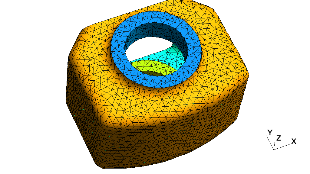
// -----------------------------------------------------------------------------
//
//  Gmsh GEO tutorial 13
//
//  Remeshing an STL file without an underlying CAD model
//
// -----------------------------------------------------------------------------

// Let's merge an STL mesh that we would like to remesh.
Merge "t13_data.stl";

// We first classify ("color") the surfaces by splitting the original surface
// along sharp geometrical features. This will create new discrete surfaces,
// curves and points.

DefineConstant[
  // Angle between two triangles above which an edge is considered as sharp
  angle = {40, Min 20, Max 120, Step 1,
    Name "Parameters/Angle for surface detection"},
  // For complex geometries, patches can be too complex, too elongated or too
  // large to be parametrized; setting the following option will force the
  // creation of patches that are amenable to reparametrization:
  forceParametrizablePatches = {0, Choices{0,1},
    Name "Parameters/Create surfaces guaranteed to be parametrizable"},
  // For open surfaces include the boundary edges in the classification process:
  includeBoundary = 1,
  // Force curves to be split on given angle:
  curveAngle = 180
];
ClassifySurfaces{angle * Pi/180, includeBoundary, forceParametrizablePatches,
                 curveAngle * Pi / 180};

// Create a geometry for all the discrete curves and surfaces in the mesh, by
// computing a parametrization for each one
CreateGeometry;

// In batch mode the two steps above can be performed with `gmsh t13.stl
// -reparam 40', which will save `t13.msh' containing the parametrizations, and
// which can thus subsequently be remeshed.

// Note that if a CAD model (e.g. as a STEP file, see `t20.geo') is available
// instead of an STL mesh, it is usually better to use that CAD model instead of
// the geometry created by reparametrizing the mesh. Indeed, CAD geometries will
// in general be more accurate, with smoother parametrizations, and will lead to
// more efficient and higher quality meshing. Discrete surface remeshing in Gmsh
// is optimized to handle dense STL meshes coming from e.g. imaging systems
// where no CAD is available; it is less well suited for the poor quality STL
// triangulations (optimized for size, with e.g. very elongated triangles) that
// are usually generated by CAD tools for e.g. 3D printing.

// Create a volume as usual
Surface Loop(1) = Surface{:};
Volume(1) = {1};

// We specify element sizes imposed by a size field, just because we can :-)
funny = DefineNumber[0, Choices{0,1},
  Name "Parameters/Apply funny mesh size field?" ];

Field[1] = MathEval;
If(funny)
  Field[1].F = "2*Sin((x+y)/5) + 3";
Else
  Field[1].F = "4";
EndIf
Background Field = 1;
2.14 t14: Homology and cohomology computation 
See t14.geo. Also available in C++ (t14.cpp), Python (t14.py), Julia (t14.jl) and Fortran (t14.f90).
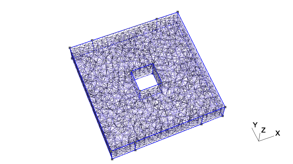
// -----------------------------------------------------------------------------
//
//  Gmsh GEO tutorial 14
//
//  Homology and cohomology computation
//
// -----------------------------------------------------------------------------

// Homology computation in Gmsh finds representative chains of (relative)
// (co)homology space bases using a mesh of a model.  The representative basis
// chains are stored in the mesh as physical groups of Gmsh, one for each chain.

// Create an example geometry

m = 0.5; // mesh size
h = 2; // height in the z-direction

Point(1) = {0, 0, 0, m};   Point(2) = {10, 0, 0, m};
Point(3) = {10, 10, 0, m}; Point(4) = {0, 10, 0, m};
Point(5) = {4, 4, 0, m};   Point(6) = {6, 4, 0, m};
Point(7) = {6, 6, 0, m};   Point(8) = {4, 6, 0, m};

Point(9) = {2, 0, 0, m};   Point(10) = {8, 0, 0, m};
Point(11) = {2, 10, 0, m}; Point(12) = {8, 10, 0, m};

Line(1) = {1, 9};  Line(2) = {9, 10}; Line(3) = {10, 2};
Line(4) = {2, 3};  Line(5) = {3, 12}; Line(6) = {12, 11};
Line(7) = {11, 4}; Line(8) = {4, 1};  Line(9) = {5, 6};
Line(10) = {6, 7}; Line(11) = {7, 8}; Line(12) = {8, 5};

Curve Loop(13) = {6, 7, 8, 1, 2, 3, 4, 5};
Curve Loop(14) = {11, 12, 9, 10};
Plane Surface(15) = {13, 14};

e() = Extrude {0, 0, h}{ Surface{15}; };

// Create physical groups, which are used to define the domain of the
// (co)homology computation and the subdomain of the relative (co)homology
// computation.

// Whole domain
Physical Volume(1) = {e(1)};

// Four "terminals" of the model
Physical Surface(70) = {e(3)};
Physical Surface(71) = {e(5)};
Physical Surface(72) = {e(7)};
Physical Surface(73) = {e(9)};

// Whole domain surface
bnd() = Boundary{ Volume{e(1)}; };
Physical Surface(80) = bnd();

// Complement of the domain surface with respect to the four terminals
bnd() -= {e(3), e(5), e(7), e(9)};
Physical Surface(75) = bnd();

// Find bases for relative homology spaces of the domain modulo the four
// terminals.
Homology {{1}, {70, 71, 72, 73}};

// Find homology space bases isomorphic to the previous bases: homology spaces
// modulo the non-terminal domain surface, a.k.a the thin cuts.
Homology {{1}, {75}};

// Find cohomology space bases isomorphic to the previous bases: cohomology
// spaces of the domain modulo the four terminals, a.k.a the thick cuts.
Cohomology {{1}, {70, 71, 72, 73}};

// More examples:
//  Homology {1};
//  Homology;
//  Homology {{1}, {80}};
//  Homology {{}, {80}};

// For more information, see M. Pellikka, S. Suuriniemi, L. Kettunen and
// C. Geuzaine. Homology and cohomology computation in finite element
// modeling. SIAM Journal on Scientific Computing 35(5), pp. 1195-1214, 2013.
2.15 t15: Embedded points, lines and surfaces 
See t15.geo. Also available in C++ (t15.cpp), Python (t15.py), Julia (t15.jl) and Fortran (t15.f90).
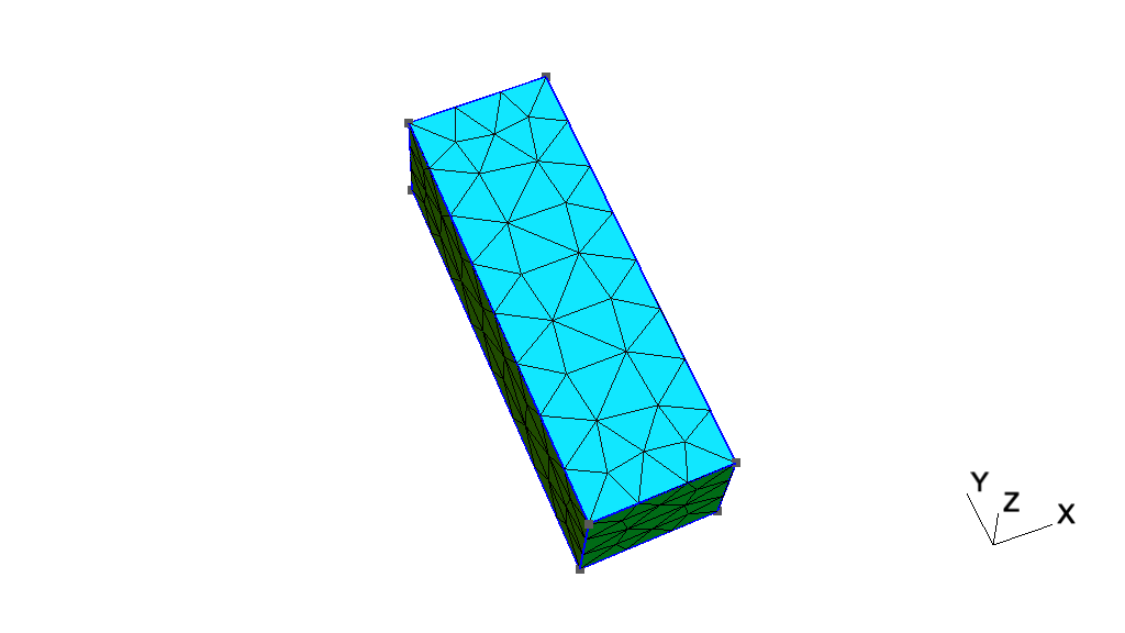
// -----------------------------------------------------------------------------
//
//  Gmsh GEO tutorial 15
//
//  Embedded points, lines and surfaces
//
// -----------------------------------------------------------------------------

// By default, across geometrical dimensions meshes generated by Gmsh are only
// conformal if lower dimensional entities are on the boundary of higher
// dimensional ones (i.e. if points, curves or surfaces are part of the boundary
// of volumes).

// Embedding constraints allow to force a mesh to be conformal to other lower
// dimensional entities.

// We start one again by including the first tutorial:
Include "t1.geo";

// We change the mesh size to generate coarser mesh
lc = lc * 4;
MeshSize {1:4} = lc;

// We define a new point
Point(5) = {0.02, 0.02, 0, lc};

// One can force this point to be included ("embedded") in the 2D mesh, using
// the `Point In Surface' command:
Point{5} In Surface{1};

// In the same way, one can force a curve to be embedded in the 2D mesh using
// the `Curve in Surface' command:
Point(6) = {0.02, 0.12, 0, lc};
Point(7) = {0.04, 0.18, 0, lc};
Line(5) = {6, 7};
Curve{5} In Surface{1};

// One can also embed points and curves in a volume using the `Curve/Point In
// Volume' commands:
Extrude {0, 0, 0.1}{ Surface {1}; }

p = newp;
Point(p) = {0.07, 0.15, 0.025, lc};
Point{p} In Volume {1};

l = newc;
Point(p+1) = {0.025, 0.15, 0.025, lc};
Line(l) = {7, p+1};
Curve{l} In Volume {1};

// Finally, one can also embed a surface in a volume using the `Surface In
// Volume' command:
Point(p+2) = {0.02, 0.12, 0.05, lc};
Point(p+3) = {0.04, 0.12, 0.05, lc};
Point(p+4) = {0.04, 0.18, 0.05, lc};
Point(p+5) = {0.02, 0.18, 0.05, lc};
Line(l+1) = {p+2, p+3};
Line(l+2) = {p+3, p+4};
Line(l+3) = {p+4, p+5};
Line(l+4) = {p+5, p+2};
ll = newcl;
Curve Loop(ll) = {l+1:l+4};
s = news;
Plane Surface(s) = {ll};
Surface{s} In Volume {1};

// Note that with the OpenCASCADE kernel (see `t16.geo'), when the
// `BooleanFragments' command is applied to entities of different dimensions,
// the lower dimensional entities will be autmatically embedded in the higher
// dimensional entities if necessary.

Physical Point("Embedded point") = {p};
Physical Curve("Embdded curve") = {l};
Physical Surface("Embedded surface") = {s};
Physical Volume("Volume") = {1};
2.16 t16: Constructive Solid Geometry, OpenCASCADE geometry kernel 
See t16.geo. Also available in C++ (t16.cpp), C (t16.c), Python (t16.py), Julia (t16.jl) and Fortran (t16.f90).
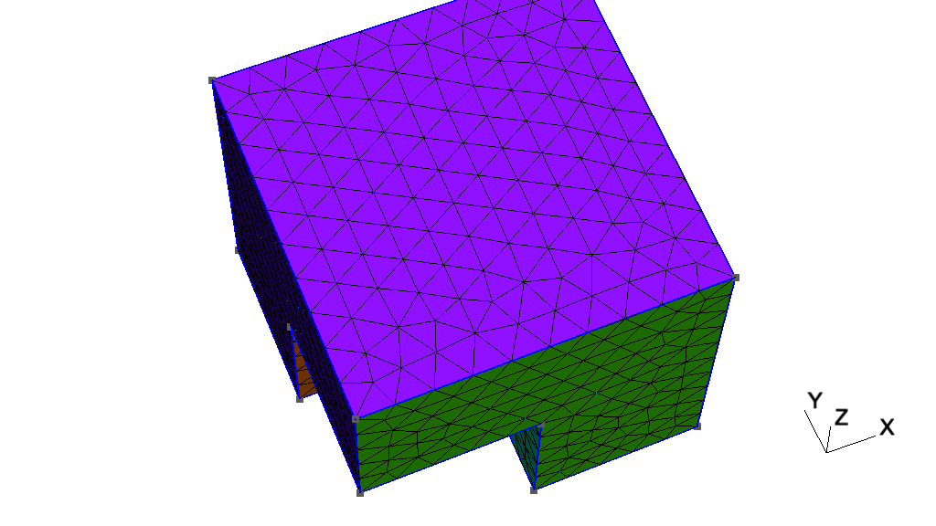
// -----------------------------------------------------------------------------
//
//  Gmsh GEO tutorial 16
//
//  Constructive Solid Geometry, OpenCASCADE geometry kernel
//
// -----------------------------------------------------------------------------

// Instead of constructing a model in a bottom-up fashion with Gmsh's built-in
// geometry kernel, starting with version 3 Gmsh allows you to directly use
// alternative geometry kernels. Here we use the OpenCASCADE kernel:

SetFactory("OpenCASCADE");

// Let's build the same model as in `t5.geo', but using constructive solid
// geometry.

// We first create two cubes:
Box(1) = {0,0,0, 1,1,1};
Box(2) = {0,0,0, 0.5,0.5,0.5};

// We apply a boolean difference to create the "cube minus one eighth" shape:
BooleanDifference(3) = { Volume{1}; Delete; }{ Volume{2}; Delete; };

// Boolean operations with OpenCASCADE always create new entities. Adding
// `Delete' in the arguments allows to automatically delete the original
// entities.

// We then create the five spheres:
x = 0 ; y = 0.75 ; z = 0 ; r = 0.09 ;
For t In {1:5}
  x += 0.166 ;
  z += 0.166 ;
  Sphere(3 + t) = {x,y,z,r};
  Physical Volume(t) = {3 + t};
EndFor

// If we had wanted five empty holes we would have used `BooleanDifference'
// again. Here we want five spherical inclusions, whose mesh should be conformal
// with the mesh of the cube: we thus use `BooleanFragments', which intersects
// all volumes in a conformal manner (without creating duplicate interfaces):
v() = BooleanFragments{ Volume{3}; Delete; }{ Volume{3 + 1 : 3 + 5}; Delete; };

// When the boolean operation leads to simple modifications of entities, and if
// one deletes the original entities with `Delete', Gmsh tries to assign the
// same tag to the new entities. (This behavior is governed by the
// `Geometry.OCCBooleanPreserveNumbering' option.)

// Here the `Physical Volume' definitions made above will thus still work, as
// the five spheres (volumes 4, 5, 6, 7 and 8), which will be deleted by the
// fragment operations, will be recreated identically (albeit with new surfaces)
// with the same tags.

// The tag of the cube will change though, so we need to access it
// programmatically:
Physical Volume(10) = v(0);

// Creating entities using constructive solid geometry is very powerful, but can
// lead to practical issues for e.g. setting mesh sizes at points, or
// identifying boundaries.

// To identify points or other bounding entities you can take advantage of the
// `CombinedBoundary`, `Closest', `PointsOf' and `In BoundingBox' commands.

// Define a physical surface for the top and right-most surfaces, by finding
// amongst the surfaces making up the boundary of the model, the two closest to
// point (1,1,0.5):
bnd() = CombinedBoundary{ Volume{:}; };
closest() = Closest {1,1,0.5} { Surface{bnd()}; };
Physical Surface("Top & right surfaces", 100) = {closest(0), closest(1)};

// Assign a mesh size to all the points of all the volumes:
lcar1 = .1;
lcar2 = .0005;
lcar3 = .055;
MeshSize{ PointsOf{ Volume{:}; } } = lcar1;

// Override this constraint on the points of the five spheres:
MeshSize{ PointsOf{ Volume{3 + 1 : 3 + 5}; } } = lcar3;

// Select the corner point by searching for it geometrically using a bounding
// box (`Closest' could have been used as well):
eps = 1e-3;
p() = Point In BoundingBox{0.5-eps, 0.5-eps, 0.5-eps,
                           0.5+eps, 0.5+eps, 0.5+eps};
MeshSize{ p() } = lcar2;

// Additional examples created with the OpenCASCADE geometry kernel are
// available in `t18.geo', `t19.geo' and `t20.geo', as well as in the
// `examples/boolean' directory.
2.17 t17: Anisotropic background mesh 
See t17.geo. Also available in C++ (t17.cpp), Python (t17.py), Julia (t17.jl) and Fortran (t17.f90).
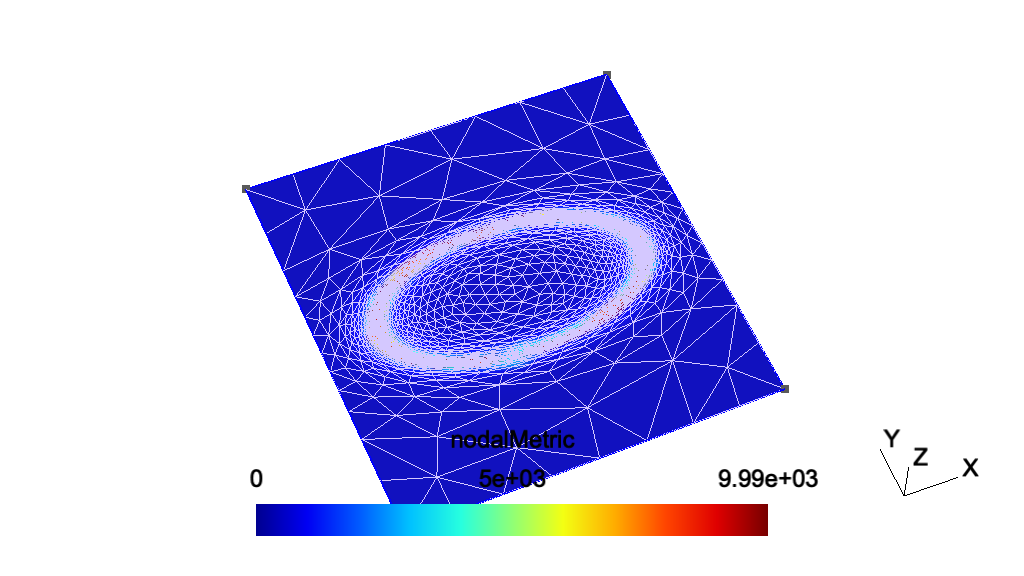
// -----------------------------------------------------------------------------
//
//  Gmsh GEO tutorial 17
//
//  Anisotropic background mesh
//
// -----------------------------------------------------------------------------

// As seen in `t7.geo', mesh sizes can be specified very accurately by providing
// a background mesh, i.e., a post-processing view that contains the target mesh
// sizes.

// Here, the background mesh is represented as a metric tensor field defined on
// a square. One should use bamg as 2d mesh generator to enable anisotropic
// meshes in 2D.

SetFactory("OpenCASCADE");

// Create a square
Rectangle(1) = {-2, -2, 0, 4, 4};

// Merge a post-processing view containing the target anisotropic mesh sizes
Merge "t17_bgmesh.pos";

// Apply the view as the current background mesh
Background Mesh View[0];

// Use bamg
Mesh.SmoothRatio = 3;
Mesh.AnisoMax = 1000;
Mesh.Algorithm = 7;
2.18 t18: Periodic meshes 
See t18.geo. Also available in C++ (t18.cpp), Python (t18.py), Julia (t18.jl) and Fortran (t18.f90).
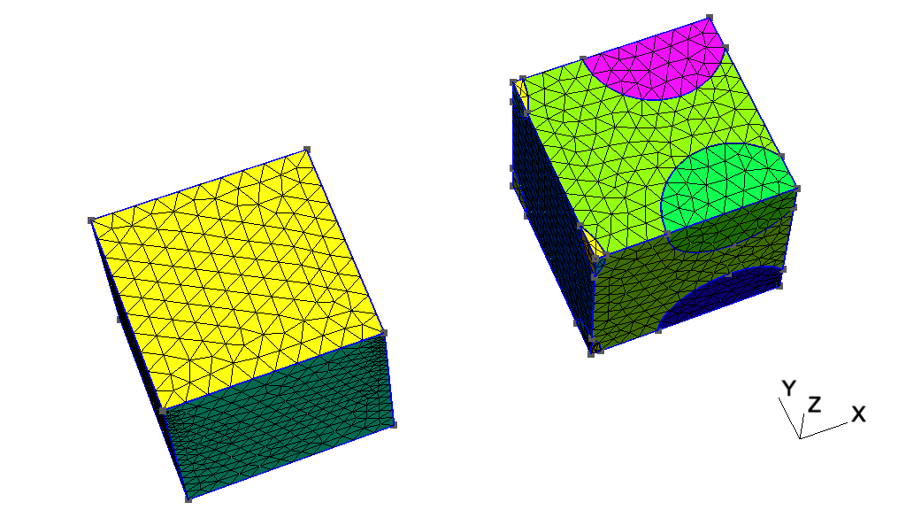
// -----------------------------------------------------------------------------
//
//  Gmsh GEO tutorial 18
//
//  Periodic meshes
//
// -----------------------------------------------------------------------------

// Periodic meshing constraints can be imposed on surfaces and curves.

// Let's use the OpenCASCADE geometry kernel to build two geometries.

SetFactory("OpenCASCADE");

// The first geometry is very simple: a unit cube with a non-uniform mesh size
// constraint (set on purpose to be able to verify visually that the periodicity
// constraint works!):

Box(1) = {0, 0, 0, 1, 1, 1};
MeshSize {:} = 0.1;
MeshSize {1} = 0.02;

// To impose that the mesh on surface 2 (the right side of the cube) should
// match the mesh from surface 1 (the left side), the following periodicity
// constraint is set:
Periodic Surface {2} = {1} Translate {1, 0, 0};

// During mesh generation, the mesh on surface 2 will be created by copying the
// mesh from surface 1.  Periodicity constraints can be specified with a
// `Translation', a `Rotation' or a general `Affine' transform.

// Multiple periodicities can be imposed in the same way:
Periodic Surface {6} = {5} Translate {0, 0, 1};
Periodic Surface {4} = {3} Translate {0, 1, 0};

// For more complicated cases, finding the corresponding surfaces by hand can be
// tedious, especially when geometries are created through solid
// modelling. Let's construct a slightly more complicated geometry.

// We start with a cube and some spheres:
Box(10) = {2, 0, 0, 1, 1, 1};
x = 2-0.3; y = 0; z = 0;
Sphere(11) = {x, y, z, 0.35};
Sphere(12) = {x+1, y, z, 0.35};
Sphere(13) = {x, y+1, z, 0.35};
Sphere(14) = {x, y, z+1, 0.35};
Sphere(15) = {x+1, y+1, z, 0.35};
Sphere(16) = {x, y+1, z+1, 0.35};
Sphere(17) = {x+1, y, z+1, 0.35};
Sphere(18) = {x+1, y+1, z+1, 0.35};

// We first fragment all the volumes, which will leave parts of spheres
// protruding outside the cube:
v() = BooleanFragments { Volume{10}; Delete; }{ Volume{11:18}; Delete; };

// Ask OpenCASCADE to compute more accurate bounding boxes of entities using the
// STL mesh:
Geometry.OCCBoundsUseStl = 1;

// We then retrieve all the volumes in the bounding box of the original cube,
// and delete all the parts outside it:
eps = 1e-3;
vin() = Volume In BoundingBox {2-eps,-eps,-eps, 2+1+eps,1+eps,1+eps};
v() -= vin();
Recursive Delete{ Volume{v()}; }

// We now set a non-uniform mesh size constraint (again to check results
// visually):
MeshSize { PointsOf{ Volume{vin()}; }} = 0.1;
p() = Point In BoundingBox{2-eps, -eps, -eps, 2+eps, eps, eps};
MeshSize {p()} = 0.001;

// We now identify corresponding surfaces on the left and right sides of the
// geometry automatically.

// First we get all surfaces on the left:
Sxmin() = Surface In BoundingBox{2-eps, -eps, -eps, 2+eps, 1+eps, 1+eps};

For i In {0:#Sxmin()-1}
  // Then we get the bounding box of each left surface
  bb() = BoundingBox Surface { Sxmin(i) };
  // We translate the bounding box to the right and look for surfaces inside it:
  Sxmax() = Surface In BoundingBox { bb(0)-eps+1, bb(1)-eps, bb(2)-eps,
                                     bb(3)+eps+1, bb(4)+eps, bb(5)+eps };
  // For all the matches, we compare the corresponding bounding boxes...
  For j In {0:#Sxmax()-1}
    bb2() = BoundingBox Surface { Sxmax(j) };
    bb2(0) -= 1;
    bb2(3) -= 1;
    // ...and if they match, we apply the periodicity constraint
    If(Fabs(bb2(0)-bb(0)) < eps && Fabs(bb2(1)-bb(1)) < eps &&
       Fabs(bb2(2)-bb(2)) < eps && Fabs(bb2(3)-bb(3)) < eps &&
       Fabs(bb2(4)-bb(4)) < eps && Fabs(bb2(5)-bb(5)) < eps)
      Periodic Surface {Sxmax(j)} = {Sxmin(i)} Translate {1,0,0};
    EndIf
  EndFor
EndFor
2.19 t19: Thrusections, fillets, pipes, mesh size from curvature 
See t19.geo. Also available in C++ (t19.cpp), Python (t19.py), Julia (t19.jl) and Fortran (t19.f90).
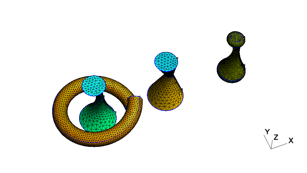
// -----------------------------------------------------------------------------
//
//  Gmsh GEO tutorial 19
//
//  Thrusections, fillets, pipes, mesh size from curvature
//
// -----------------------------------------------------------------------------

// The OpenCASCADE geometry kernel supports several useful features for solid
// modelling.

SetFactory("OpenCASCADE");

// Volumes can be constructed from (closed) curve loops thanks to the
// `ThruSections' command
Circle(1) = {0,0,0, 0.5};       Curve Loop(1) = 1;
Circle(2) = {0.1,0.05,1, 0.1};  Curve Loop(2) = 2;
Circle(3) = {-0.1,-0.1,2, 0.3}; Curve Loop(3) = 3;
ThruSections(1) = {1:3};

// With `Ruled ThruSections' you can force the use of ruled surfaces:
Circle(11) = {2+0,0,0, 0.5};      Curve Loop(11) = 11;
Circle(12) = {2+0.1,0.05,1, 0.1}; Curve Loop(12) = 12;
Circle(13) = {2-0.1,-0.1,2, 0.3}; Curve Loop(13) = 13;
Ruled ThruSections(11) = {11:13};

// We copy the first volume, and fillet all its edges:
v() = Translate{4, 0, 0} { Duplicata{ Volume{1}; } };
f() = Boundary{ Volume{v(0)}; };
e() = Unique(Boundary{ Surface{f()}; });
Fillet{v(0)}{e()}{0.1}

// OpenCASCADE also allows general extrusions along a smooth path. Let's first
// define a spline curve:
nturns = 1;
npts = 20;
r = 1;
h = 1 * nturns;
For i In {0 : npts - 1}
  theta = i * 2*Pi*nturns/npts;
  Point(1000 + i) = {r * Cos(theta), r * Sin(theta), i * h/npts};
EndFor
Spline(1000) = {1000 : 1000 + npts - 1};

// A wire is like a curve loop, but open:
Wire(1000) = {1000};

// We define the shape we would like to extrude along the spline (a disk):
Disk(1000) = {1,0,0, 0.2};
Rotate {{1, 0, 0}, {0, 0, 0}, Pi/2} { Surface{1000}; }

// We extrude the disk along the spline to create a pipe:
Extrude { Surface{1000}; } Using Wire {1000}

// We delete the source surface, and increase the number of sub-edges for a
// nicer display of the geometry:
Delete{ Surface{1000}; }
Geometry.NumSubEdges = 1000;

// We can activate the calculation of mesh element sizes based on curvature
// (here with a target of 20 elements per 2*Pi radians):
Mesh.MeshSizeFromCurvature = 20;

// We can constraint the min and max element sizes to stay within reasonnable
// values (see `t10.geo' for more details):
Mesh.MeshSizeMin = 0.001;
Mesh.MeshSizeMax = 0.3;
2.20 t20: STEP import and manipulation, geometry partitioning 
See t20.geo. Also available in C++ (t20.cpp), Python (t20.py), Julia (t20.jl) and Fortran (t20.f90).
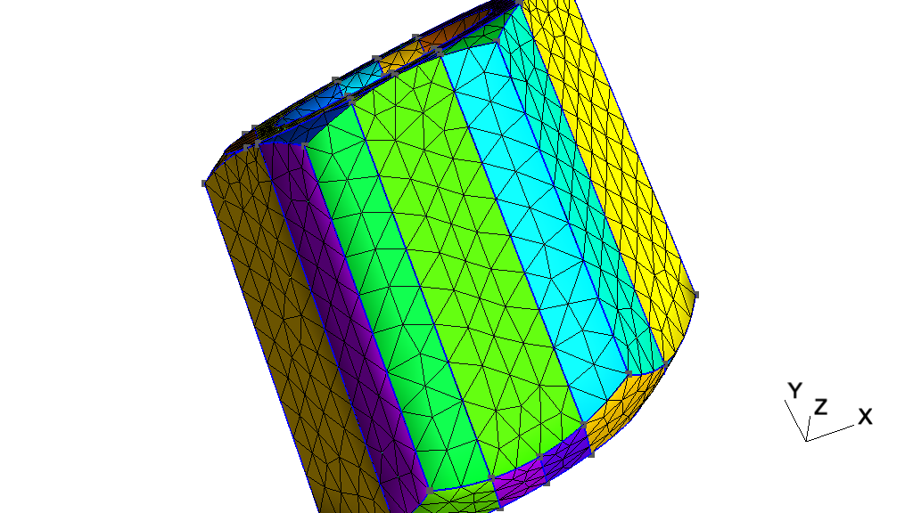
// -----------------------------------------------------------------------------
//
//  Gmsh GEO tutorial 20
//
//  STEP import and manipulation, geometry partitioning
//
// -----------------------------------------------------------------------------

// The OpenCASCADE geometry kernel allows to import STEP files and to modify
// them. In this tutorial we will load a STEP geometry and partition it into
// slices.

SetFactory("OpenCASCADE");

// Load a STEP file (using `ShapeFromFile' instead of `Merge' allows to directly
// retrieve the tags of the highest dimensional imported entities):
v() = ShapeFromFile("t20_data.step");

// If we had specified
//
// Geometry.OCCTargetUnit = "M";
//
// before merging the STEP file, OpenCASCADE would have converted the units to
// meters (instead of the default, which is millimeters).

// Get the bounding box of the volume:
bbox() = BoundingBox Volume{v()};
xmin = bbox(0);
ymin = bbox(1);
zmin = bbox(2);
xmax = bbox(3);
ymax = bbox(4);
zmax = bbox(5);

// We want to slice the model into N slices, and either keep the volume slices
// or just the surfaces obtained by the cutting:
DefineConstant[
  N = {5, Min 2, Max 100, Step 1, Name "Parameters/0Number of slices"}
  dir = {0, Choices{0="X", 1="Y", 2="Z"}, Name "Parameters/1Direction"}
  surf = {0, Choices{0, 1}, Name "Parameters/2Keep only surfaces?"}
];

dx = (xmax - xmin);
dy = (ymax - ymin);
dz = (zmax - zmin);
L = (dir == 0) ? dz : dx;
H = (dir == 1) ? dz : dy;

// Create the first cutting plane:
s() = {news};
Rectangle(s(0)) = {xmin, ymin, zmin, L, H};
If(dir == 0)
  Rotate{ {0, 1, 0}, {xmin, ymin, zmin}, -Pi/2 } { Surface{s(0)}; }
ElseIf(dir == 1)
  Rotate{ {1, 0, 0}, {xmin, ymin, zmin}, Pi/2 } { Surface{s(0)}; }
EndIf
tx = (dir == 0) ? dx / N : 0;
ty = (dir == 1) ? dy / N : 0;
tz = (dir == 2) ? dz / N : 0;
Translate{tx, ty, tz} { Surface{s(0)}; }

// Create the other cutting planes:
For i In {1:N-2}
  s() += Translate{i * tx, i * ty, i * tz} { Duplicata{ Surface{s(0)}; } };
EndFor

// Fragment (i.e. intersect) the volume with all the cutting planes:
BooleanFragments{ Volume{v()}; Delete; }{ Surface{s()}; Delete; }

// Now remove all the surfaces (and their bounding entities) that are not on the
// boundary of a volume, i.e. the parts of the cutting planes that "stick out"
// of the volume:
Recursive Delete { Surface{:}; }

If(surf)
  // If we want to only keep the surfaces, retrieve the surfaces in bounding
  // boxes around the cutting planes...
  eps = 1e-4;
  s() = {};
  For i In {1:N-1}
    xx = (dir == 0) ? xmin : xmax;
    yy = (dir == 1) ? ymin : ymax;
    zz = (dir == 2) ? zmin : zmax;
    s() += Surface In BoundingBox
      {xmin - eps + i * tx, ymin - eps + i * ty, zmin - eps + i * tz,
       xx + eps + i * tx, yy + eps + i * ty, zz + eps + i * tz};
  EndFor
  // ...and remove all the other entities:
  dels = Surface{:};
  dels -= s();
  Delete { Volume{:}; Surface{dels()}; Curve{:}; Point{:}; }
EndIf

// Finally, let's specify a global mesh size:
Mesh.MeshSizeMin = 3;
Mesh.MeshSizeMax = 3;

// To partition the mesh instead of the geometry, see `t21.geo'.
2.21 t21: Mesh partitioning 
See t21.geo. Also available in C++ (t21.cpp), Python (t21.py), Julia (t21.jl) and Fortran (t21.f90).
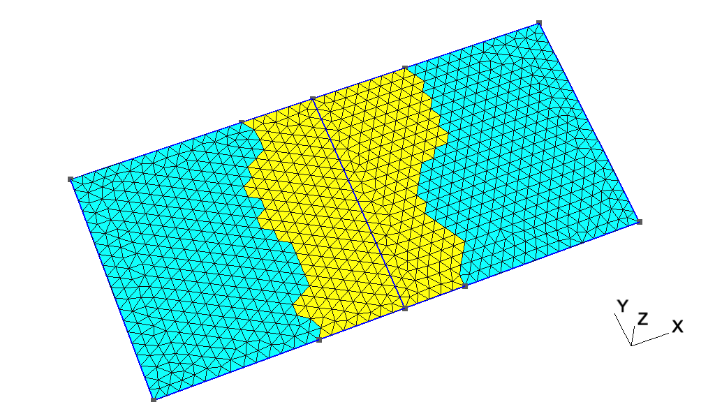
// -----------------------------------------------------------------------------
//
//  Gmsh GEO tutorial 21
//
//  Mesh partitioning
//
// -----------------------------------------------------------------------------

// Gmsh can partition meshes using different algorithms, e.g. the graph
// partitioner Metis or the `SimplePartition' plugin. For all the partitioning
// algorithms, the relationship between mesh elements and mesh partitions is
// encoded through the creation of new (discrete) elementary entities, called
// "partition entities".
//
// Partition entities behave exactly like other discrete elementary entities;
// the only difference is that they keep track of both a mesh partition index
// and their parent elementary entity.
//
// The major advantage of this approach is that it allows to maintain a full
// boundary representation of the partition entities, which Gmsh creates
// automatically if `Mesh.PartitionCreateTopology' is set.

// Let us start by creating a simple geometry with two adjacent squares sharing
// an edge:
SetFactory("OpenCASCADE");
Rectangle(1) = {0, 0, 0, 1, 1};
Rectangle(2) = {1, 0, 0, 1, 1};
BooleanFragments{ Surface{1}; Delete; }{ Surface{2}; Delete; }
MeshSize {:} = 0.05;

// We create one physical group for each square, and we mesh the resulting
// geometry:
Physical Surface("Left", 100) = 1;
Physical Surface("Right", 200) = 2;
Mesh 2;

// We now define several constants to fine-tune how the mesh will be partitioned
DefineConstant[
  partitioner = {0, Choices{0="Metis", 1="SimplePartition"},
    Name "Parameters/0Mesh partitioner"}
  N = {3, Min 1, Max 256, Step 1,
    Name "Parameters/1Number of partitions"}
  topology = {1, Choices{0, 1},
    Name "Parameters/2Create partition topology (BRep)?"}
  ghosts = {0, Choices{0, 1},
    Name "Parameters/3Create ghost cells?"}
  physicals = {0, Choices{0, 1},
    Name "Parameters/3Create new physical groups?"}
  write = {1, Choices {0, 1},
    Name "Parameters/3Write file to disk?"}
  split = {0, Choices {0, 1},
    Name "Parameters/4Write one file per partition?"}
];

// Should we create the boundary representation of the partition entities?
Mesh.PartitionCreateTopology = topology;

// Should we create ghost cells?
Mesh.PartitionCreateGhostCells = ghosts;

// Should we automatically create new physical groups on the partition entities?
Mesh.PartitionCreatePhysicals = physicals;

// Should we keep backward compatibility with pre-Gmsh 4, e.g. to save the mesh
// in MSH2 format?
Mesh.PartitionOldStyleMsh2 = 0;

// Should we save one mesh file per partition?
Mesh.PartitionSplitMeshFiles = split;

If (partitioner == 0)
  // Use Metis to create N partitions
  PartitionMesh N;
  // Several options can be set to control Metis: `Mesh.MetisAlgorithm' (1:
  // Recursive, 2: K-way), `Mesh.MetisObjective' (1: min. edge-cut, 2:
  // min. communication volume), `Mesh.PartitionTriWeight' (weight of
  // triangles), `Mesh.PartitionQuadWeight' (weight of quads), ...
Else
  // Use the `SimplePartition' plugin to create chessboard-like partitions
  Plugin(SimplePartition).NumSlicesX = N;
  Plugin(SimplePartition).NumSlicesY = 1;
  Plugin(SimplePartition).NumSlicesZ = 1;
  Plugin(SimplePartition).Run;
EndIf

// Save mesh file (or files, if `Mesh.PartitionSplitMeshFiles' is set):
If(write)
  Save "t21.msh";
EndIf
2.22 x1: Geometry and mesh data 
See x1.py. Also available in C++ (x1.cpp) and Julia (x1.jl).
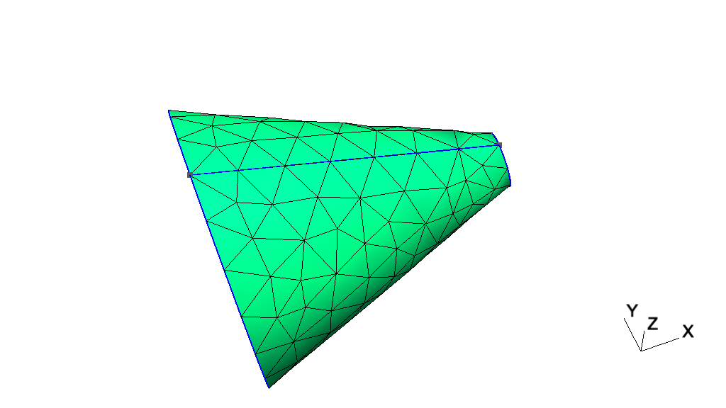
# -----------------------------------------------------------------------------
#
#  Gmsh Python extended tutorial 1
#
#  Geometry and mesh data
#
# -----------------------------------------------------------------------------

# The Python API allows to do much more than what can be done in .geo
# files. These additional features are introduced gradually in the extended
# tutorials, starting with `x1.py'.

# In this first extended tutorial, we start by using the API to access basic
# geometrical and mesh data.

import gmsh
import sys

gmsh.initialize()

if len(sys.argv) > 1 and sys.argv[1][0] != '-':
    # If an argument is provided, handle it as a file that Gmsh can read, e.g. a
    # mesh file in the MSH format (`python x1.py file.msh')
    gmsh.open(sys.argv[1])
else:
    # Otherwise, create and mesh a simple geometry
    gmsh.model.occ.addCone(1, 0, 0, 1, 0, 0, 0.5, 0.1)
    gmsh.model.occ.synchronize()
    gmsh.model.mesh.generate()

# Print the model name and dimension:
print('Model ' + gmsh.model.getCurrent() + ' (' +
      str(gmsh.model.getDimension()) + 'D)')

# Geometrical data is made of elementary model `entities', called `points'
# (entities of dimension 0), `curves' (entities of dimension 1), `surfaces'
# (entities of dimension 2) and `volumes' (entities of dimension 3). As we have
# seen in the other Python tutorials, elementary model entities are identified
# by their dimension and by a `tag': a strictly positive identification
# number. Model entities can be either CAD entities (from the built-in `geo'
# kernel or from the OpenCASCADE `occ' kernel) or `discrete' entities (defined
# by a mesh). `Physical groups' are collections of model entities and are also
# identified by their dimension and by a tag.

# Get all the elementary entities in the model, as a vector of (dimension, tag)
# pairs:
entities = gmsh.model.getEntities()

for e in entities:
    # Dimension and tag of the entity:
    dim = e[0]
    tag = e[1]

    # Mesh data is made of `elements' (points, lines, triangles, ...), defined
    # by an ordered list of their `nodes'. Elements and nodes are identified by
    # `tags' as well (strictly positive identification numbers), and are stored
    # ("classified") in the model entity they discretize. Tags for elements and
    # nodes are globally unique (and not only per dimension, like entities).

    # A model entity of dimension 0 (a geometrical point) will contain a mesh
    # element of type point, as well as a mesh node. A model curve will contain
    # line elements as well as its interior nodes, while its boundary nodes will
    # be stored in the bounding model points. A model surface will contain
    # triangular and/or quadrangular elements and all the nodes not classified
    # on its boundary or on its embedded entities. A model volume will contain
    # tetrahedra, hexahedra, etc. and all the nodes not classified on its
    # boundary or on its embedded entities.

    # Get the mesh nodes for the entity (dim, tag):
    nodeTags, nodeCoords, nodeParams = gmsh.model.mesh.getNodes(dim, tag)

    # Get the mesh elements for the entity (dim, tag):
    elemTypes, elemTags, elemNodeTags = gmsh.model.mesh.getElements(dim, tag)

    # Elements can also be obtained by type, by using `getElementTypes()'
    # followed by `getElementsByType()'.

    # Let's print a summary of the information available on the entity and its
    # mesh.

    # * Type and name of the entity:
    type = gmsh.model.getType(dim, tag)
    name = gmsh.model.getEntityName(dim, tag)
    if len(name): name += ' '
    print("Entity " + name + str(e) + " of type " + type)

    # * Number of mesh nodes and elements:
    numElem = sum(len(i) for i in elemTags)
    print(" - Mesh has " + str(len(nodeTags)) + " nodes and " + str(numElem) +
          " elements")

    # * Upward and downward adjacencies:
    up, down = gmsh.model.getAdjacencies(dim, tag)
    if len(up):
        print(" - Upward adjacencies: " + str(up))
    if len(down):
        print(" - Downward adjacencies: " + str(down))

    # * Does the entity belong to physical groups?
    physicalTags = gmsh.model.getPhysicalGroupsForEntity(dim, tag)
    if len(physicalTags):
        s = ''
        for p in physicalTags:
            n = gmsh.model.getPhysicalName(dim, p)
            if n: n += ' '
            s += n + '(' + str(dim) + ', ' + str(p) + ') '
        print(" - Physical groups: " + s)

    # * Is the entity a partition entity? If so, what is its parent entity?
    partitions = gmsh.model.getPartitions(dim, tag)
    if len(partitions):
        print(" - Partition tags: " + str(partitions) + " - parent entity " +
              str(gmsh.model.getParent(dim, tag)))

    # * List all types of elements making up the mesh of the entity:
    for t in elemTypes:
        name, dim, order, numv, parv, _ = gmsh.model.mesh.getElementProperties(
            t)
        print(" - Element type: " + name + ", order " + str(order) + " (" +
              str(numv) + " nodes in param coord: " + str(parv) + ")")

# Launch the GUI to see the model:
if '-nopopup' not in sys.argv:
    gmsh.fltk.run()

# We can use this to clear all the model data:
gmsh.clear()

gmsh.finalize()
2.23 x2: Mesh import, discrete entities, hybrid models, terrain meshing 
See x2.py. Also available in C++ (x2.cpp) and Julia (x2.jl).
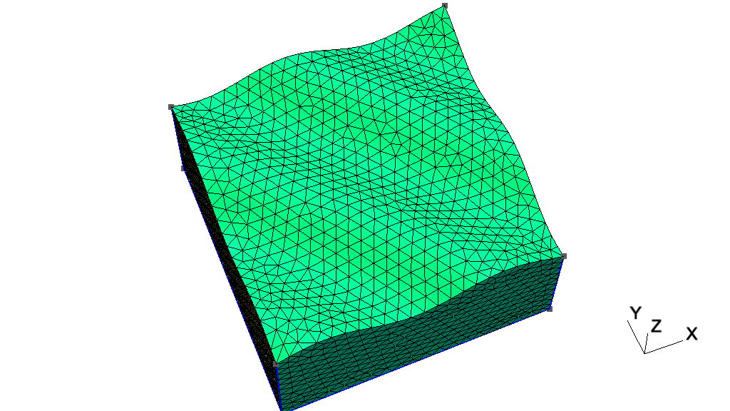
# -----------------------------------------------------------------------------
#
#  Gmsh Python extended tutorial 2
#
#  Mesh import, discrete entities, hybrid models, terrain meshing
#
# -----------------------------------------------------------------------------

import gmsh
import sys
import math

# The API can be used to import a mesh without reading it from a file, by
# creating nodes and elements on the fly and storing them in model
# entities. These model entities can be existing CAD entities, or can be
# discrete entities, entirely defined by the mesh.
#
# Discrete entities can be reparametrized (see `t13.py') so that they can be
# remeshed later on; and they can also be combined with built-in CAD entities to
# produce hybrid models.
#
# We combine all these features in this tutorial to perform terrain meshing,
# where the terrain is described by a discrete surface (that we then
# reparametrize) combined with a CAD representation of the underground.

gmsh.initialize()

gmsh.model.add("x2")

# We will create the terrain surface mesh from N x N input data points:
N = 100


# Helper function to return a node tag given two indices i and j:
def tag(i, j):
    return (N + 1) * i + j + 1


# The x, y, z coordinates of all the nodes:
coords = []

# The tags of the corresponding nodes:
nodes = []

# The connectivities of the triangle elements (3 node tags per triangle) on the
# terrain surface:
tris = []

# The connectivities of the line elements on the 4 boundaries (2 node tags
# for each line element):
lin = [[], [], [], []]

# The connectivities of the point elements on the 4 corners (1 node tag for each
# point element):
pnt = [tag(0, 0), tag(N, 0), tag(N, N), tag(0, N)]

for i in range(N + 1):
    for j in range(N + 1):
        nodes.append(tag(i, j))
        coords.extend([
            float(i) / N,
            float(j) / N, 0.05 * math.sin(10 * float(i + j) / N)
        ])
        if i > 0 and j > 0:
            tris.extend([tag(i - 1, j - 1), tag(i, j - 1), tag(i - 1, j)])
            tris.extend([tag(i, j - 1), tag(i, j), tag(i - 1, j)])
        if (i == 0 or i == N) and j > 0:
            lin[3 if i == 0 else 1].extend([tag(i, j - 1), tag(i, j)])
        if (j == 0 or j == N) and i > 0:
            lin[0 if j == 0 else 2].extend([tag(i - 1, j), tag(i, j)])

# Create 4 discrete points for the 4 corners of the terrain surface:
for i in range(4):
    gmsh.model.addDiscreteEntity(0, i + 1)
gmsh.model.setCoordinates(1, 0, 0, coords[3 * tag(0, 0) - 1])
gmsh.model.setCoordinates(2, 1, 0, coords[3 * tag(N, 0) - 1])
gmsh.model.setCoordinates(3, 1, 1, coords[3 * tag(N, N) - 1])
gmsh.model.setCoordinates(4, 0, 1, coords[3 * tag(0, N) - 1])

# Create 4 discrete bounding curves, with their boundary points:
for i in range(4):
    gmsh.model.addDiscreteEntity(1, i + 1, [i + 1, i + 2 if i < 3 else 1])

# Create one discrete surface, with its bounding curves:
gmsh.model.addDiscreteEntity(2, 1, [1, 2, -3, -4])

# Add all the nodes on the surface (for simplicity... see below):
gmsh.model.mesh.addNodes(2, 1, nodes, coords)

# Add point elements on the 4 points, line elements on the 4 curves, and
# triangle elements on the surface:
for i in range(4):
    # Type 15 for point elements:
    gmsh.model.mesh.addElementsByType(i + 1, 15, [], [pnt[i]])
    # Type 1 for 2-node line elements:
    gmsh.model.mesh.addElementsByType(i + 1, 1, [], lin[i])
# Type 2 for 3-node triangle elements:
gmsh.model.mesh.addElementsByType(1, 2, [], tris)

# Reclassify the nodes on the curves and the points (since we put them all on
# the surface before with `addNodes' for simplicity)
gmsh.model.mesh.reclassifyNodes()

# Create a geometry for the discrete curves and surfaces, so that we can remesh
# them later on:
gmsh.model.mesh.createGeometry()

# Note that for more complicated meshes, e.g. for on input unstructured STL
# mesh, we could use `classifySurfaces()' to automatically create the discrete
# entities and the topology; but we would then have to extract the boundaries
# afterwards.

# Create other build-in CAD entities to form one volume below the terrain
# surface. Beware that only built-in CAD entities can be hybrid, i.e. have
# discrete entities on their boundary: OpenCASCADE does not support this
# feature.
p1 = gmsh.model.geo.addPoint(0, 0, -0.5)
p2 = gmsh.model.geo.addPoint(1, 0, -0.5)
p3 = gmsh.model.geo.addPoint(1, 1, -0.5)
p4 = gmsh.model.geo.addPoint(0, 1, -0.5)
c1 = gmsh.model.geo.addLine(p1, p2)
c2 = gmsh.model.geo.addLine(p2, p3)
c3 = gmsh.model.geo.addLine(p3, p4)
c4 = gmsh.model.geo.addLine(p4, p1)
c10 = gmsh.model.geo.addLine(p1, 1)
c11 = gmsh.model.geo.addLine(p2, 2)
c12 = gmsh.model.geo.addLine(p3, 3)
c13 = gmsh.model.geo.addLine(p4, 4)
ll1 = gmsh.model.geo.addCurveLoop([c1, c2, c3, c4])
s1 = gmsh.model.geo.addPlaneSurface([ll1])
ll3 = gmsh.model.geo.addCurveLoop([c1, c11, -1, -c10])
s3 = gmsh.model.geo.addPlaneSurface([ll3])
ll4 = gmsh.model.geo.addCurveLoop([c2, c12, -2, -c11])
s4 = gmsh.model.geo.addPlaneSurface([ll4])
ll5 = gmsh.model.geo.addCurveLoop([c3, c13, 3, -c12])
s5 = gmsh.model.geo.addPlaneSurface([ll5])
ll6 = gmsh.model.geo.addCurveLoop([c4, c10, 4, -c13])
s6 = gmsh.model.geo.addPlaneSurface([ll6])
sl1 = gmsh.model.geo.addSurfaceLoop([s1, s3, s4, s5, s6, 1])
v1 = gmsh.model.geo.addVolume([sl1])
gmsh.model.geo.synchronize()

# Set this to True to build a fully hex mesh:
#transfinite = True
transfinite = False
transfiniteAuto = False

if transfinite:
    NN = 30
    for c in gmsh.model.getEntities(1):
        gmsh.model.mesh.setTransfiniteCurve(c[1], NN)
    for s in gmsh.model.getEntities(2):
        gmsh.model.mesh.setTransfiniteSurface(s[1])
        gmsh.model.mesh.setRecombine(s[0], s[1])
        gmsh.model.mesh.setSmoothing(s[0], s[1], 100)
    gmsh.model.mesh.setTransfiniteVolume(v1)
elif transfiniteAuto:
    gmsh.option.setNumber('Mesh.MeshSizeMin', 0.5)
    gmsh.option.setNumber('Mesh.MeshSizeMax', 0.5)
    # setTransfiniteAutomatic() uses the sizing constraints to set the number
    # of points
    gmsh.model.mesh.setTransfiniteAutomatic()
else:
    gmsh.option.setNumber('Mesh.MeshSizeMin', 0.05)
    gmsh.option.setNumber('Mesh.MeshSizeMax', 0.05)

gmsh.model.mesh.generate(3)
gmsh.write('x2.msh')

# Launch the GUI to see the results:
if '-nopopup' not in sys.argv:
    gmsh.fltk.run()

gmsh.finalize()
2.24 x3: Post-processing data import: list-based 
See x3.py. Also available in C++ (x3.cpp) and Julia (x3.jl).
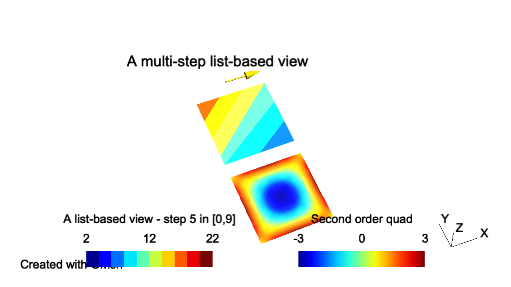
# -----------------------------------------------------------------------------
#
#  Gmsh Python extended tutorial 3
#
#  Post-processing data import: list-based
#
# -----------------------------------------------------------------------------

import gmsh
import sys

gmsh.initialize(sys.argv)

# Gmsh supports two types of post-processing data: "list-based" and
# "model-based". Both types of data are handled through the `view' interface.

# List-based views are completely independent from any model and any mesh: they
# are self-contained and simply contain lists of coordinates and values, element
# by element, for 3 types of fields (scalar "S", vector "V" and tensor "T") and
# several types of element shapes (point "P", line "L", triangle "T", quadrangle
# "Q", tetrahedron "S", hexahedron "H", prism "I" and pyramid "Y"). (See `x4.py'
# for a tutorial on model-based views.)

# To create a list-based view one should first create a view:
t1 = gmsh.view.add("A list-based view")

# List-based data is then added by specifying the type as a 2 character string
# that combines a field type and an element shape (e.g. "ST" for a scalar field
# on triangles), the number of elements to be added, and the concatenated list
# of coordinates (e.g. 3 "x" coordinates, 3 "y" coordinates, 3 "z" coordinates
# for first order triangles) and values for each element (e.g. 3 values for
# first order scalar triangles, repeated for each step if there are several time
# steps).

# Let's create two triangles...
triangle1 = [0., 1., 1., # x coordinates of the 3 triangle nodes
             0., 0., 1., # y coordinates of the 3 triangle nodes
             0., 0., 0.] # z coordinates of the 3 triangle nodes
triangle2 = [0., 1., 0., 0., 1., 1., 0., 0., 0.]

# ... and append values for 10 time steps
for step in range(0, 10):
    triangle1.extend([10., 11. - step, 12.])  # 3 node values for each step
    triangle2.extend([11., 12., 13. + step])

# List-based data is just added by concatenating the data for all the triangles:
gmsh.view.addListData(t1, "ST", 2, triangle1 + triangle2)

# Internally, post-processing views parsed by the .geo file parser create such
# list-based data (see e.g. `t7.py', `t8.py' and `t9.py'), independently of any
# mesh.

# Vector or tensor fields can be imported in the same way, the only difference
# beeing the type (starting with "V" for vector fields and "T" for tensor
# fields) and the number of components. For example a vector field on a line
# element can be added as follows:
line = [
    0., 1.,   # x coordinate of the 2 line nodes
    1.2, 1.2, # y coordinate of the 2 line nodes
    0., 0.    # z coordinate of the 2 line nodes
]
for step in range(0, 10):
    # 3 vector components for each node (2 nodes here), for each step
    line.extend([10. + step, 0., 0.,
                 10. + step, 0., 0.])
gmsh.view.addListData(t1, "VL", 1, line)

# List-based data can also hold 2D (in window coordinates) and 3D (in model
# coordinates) strings (see `t4.py'). Here we add a 2D string located on the
# bottom-left of the window (with a 20 pixels offset), as well as a 3D string
# located at model coordinates (0.5, 0.5. 0):
gmsh.view.addListDataString(t1, [20., -20.], ["Created with Gmsh"])
gmsh.view.addListDataString(t1, [0.5, 1.5, 0.],
                            ["A multi-step list-based view"],
                            ["Align", "Center", "Font", "Helvetica"])

# The various attributes of the view can be queried and changed using the option
# interface:
gmsh.view.option.setNumber(t1, "TimeStep", 5)
gmsh.view.option.setNumber(t1, "IntervalsType", 3)
ns = gmsh.view.option.getNumber(t1, "NbTimeStep")
print("View " + str(t1) + " has " + str(ns) + " time steps")

# Views can be queried and modified in various ways using plugins (see `t9.py'),
# or probed directly using `gmsh.view.probe()' - here at point (0.9, 0.1, 0):
print("Value at (0.9, 0.1, 0)", gmsh.view.probe(t1, 0.9, 0.1, 0))

# Views can be saved to disk using `gmsh.view.write()':
gmsh.view.write(t1, "x3.pos")

# High-order datasets can be provided by setting the interpolation matrices
# explicitly. Let's create a second view with second order interpolation on
# a 4-node quadrangle.

# Add a new view:
t2 = gmsh.view.add("Second order quad")

# Set the node coordinates:
quad = [0., 1., 1., 0., # x coordinates of the 4 quadrangle nodes
        -1.2, -1.2, -0.2, -0.2, # y coordinates of the 4 quadrangle nodes
        0., 0., 0., 0.] # z coordinates of the 4 quadrangle nodes

# Add nine values that will be interpolated by second order basis functions
quad.extend([1., 1., 1., 1., 3., 3., 3., 3., -3.])

# Set the two interpolation matrices c[i][j] and e[i][j] defining the d = 9
# basis functions: f[i](u, v, w) = sum_(j = 0, ..., d - 1) c[i][j] u^e[j][0]
# v^e[j][1] w^e[j][2], i = 0, ..., d-1, with u, v, w the coordinates in the
# reference element:
gmsh.view.setInterpolationMatrices(t2, "Quadrangle", 9,
                                   [0, 0, 0.25, 0, 0, -0.25, -0.25, 0, 0.25,
                                    0, 0, 0.25, 0, 0, -0.25, 0.25, 0, -0.25,
                                    0, 0, 0.25, 0, 0, 0.25, 0.25, 0, 0.25,
                                    0, 0, 0.25, 0, 0, 0.25, -0.25, 0, -0.25,
                                    0, 0, -0.5, 0.5, 0, 0.5, 0, -0.5, 0,
                                    0, 0.5, -0.5, 0, 0.5, 0, -0.5, 0, 0,
                                    0, 0, -0.5, 0.5, 0, -0.5, 0, 0.5, 0,
                                    0, 0.5, -0.5, 0, -0.5, 0, 0.5, 0, 0,
                                    1, -1, 1, -1, 0, 0, 0, 0, 0],
                                   [0, 0, 0,
                                    2, 0, 0,
                                    2, 2, 0,
                                    0, 2, 0,
                                    1, 0, 0,
                                    2, 1, 0,
                                    1, 2, 0,
                                    0, 1, 0,
                                    1, 1, 0])

# Note that two additional interpolation matrices could also be provided to
# interpolate the geometry, i.e. to interpolate curved elements.

# Add the data to the view:
gmsh.view.addListData(t2, "SQ", 1, quad)

# In order to visualize the high-order field, one must activate adaptive
# visualization, set a visualization error threshold and a maximum subdivision
# level (Gmsh does automatic mesh refinement to visualize the high-order field
# with the requested accuracy):
gmsh.view.option.setNumber(t2, "AdaptVisualizationGrid", 1)
gmsh.view.option.setNumber(t2, "TargetError", 1e-2)
gmsh.view.option.setNumber(t2, "MaxRecursionLevel", 5)

# Note that the adapted visualization data can be retrived by setting the
# `returnAdaptive' argument to the `gmsh.view.getListData()' function.

# Launch the GUI to see the results:
if '-nopopup' not in sys.argv:
    gmsh.fltk.run()

gmsh.finalize()
2.25 x4: Post-processing data import: model-based 
See x4.py. Also available in C++ (x4.cpp) and Julia (x4.jl).
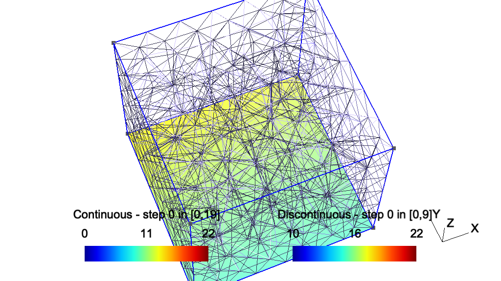
# -----------------------------------------------------------------------------
#
#  Gmsh Python extended tutorial 4
#
#  Post-processing data import: model-based
#
# -----------------------------------------------------------------------------

import gmsh
import sys

gmsh.initialize(sys.argv)

# Contrary to list-based view (see `x3.py'), model-based views are based on one
# or more meshes. Compared to list-based views, they are thus linked to one
# model (per step). Post-processing data stored in MSH files create such
# model-based views.

# Let's create a first model-based view using a simple mesh constructed by
# hand. We create a model with a discrete surface
gmsh.model.add("simple model")
surf = gmsh.model.addDiscreteEntity(2)

# We add 4 nodes and 2 3-node triangles (element type "2")
gmsh.model.mesh.addNodes(2, surf, [1, 2, 3, 4],
                         [0., 0., 0., 1., 0., 0., 1., 1., 0., 0., 1., 0.])
gmsh.model.mesh.addElementsByType(surf, 2, [1, 2], [1, 2, 3, 1, 3, 4])

# We can now create a new model-based view, to which we add 10 steps of
# node-based data:
t1 = gmsh.view.add("Continuous")
for step in range(0, 10):
    gmsh.view.addHomogeneousModelData(
        t1, step, "simple model", "NodeData",
        [1, 2, 3, 4],  # tags of nodes
        [10., 10., 12. + step, 13. + step])  # data, per node

# Besided node-based data, which result in continuous fields, one can also add
# general discontinous fields defined at the nodes of each element, using
# "ElementNodeData":
t2 = gmsh.view.add("Discontinuous")
for step in range(0, 10):
    gmsh.view.addHomogeneousModelData(
        t2, step, "simple model", "ElementNodeData",
        [1, 2],  # tags of elements
        [10., 10., 12. + step, 14., 15., 13. + step])  # data per element nodes

# Constant per element datasets can also be created using "ElementData". Note
# that a more general function `addModelData' to add data for hybrid meshes
# (when data is not homogeneous, i.e. when the number of nodes changes between
# elements) is also available.

# Each step of a model-based view can be defined on a different model, i.e. on a
# different mesh. Let's define a second model and mesh it
gmsh.model.add("another model")
gmsh.model.occ.addBox(0, 0, 0, 1, 1, 1)
gmsh.model.occ.synchronize()
gmsh.model.mesh.generate(3)

# We can add other steps to view "t" based on this new mesh:
nodes, coord, _ = gmsh.model.mesh.getNodes()
for step in range(11, 20):
    gmsh.view.addHomogeneousModelData(
        t1, step, "another model", "NodeData", nodes,
        [step * coord[i] for i in range(0, len(coord), 3)])

# This feature allows to create seamless animations for time-dependent datasets
# on deforming or remeshed models.

# High-order node-based datasets are supported without needing to supply the
# interpolation matrices (iso-parametric Lagrange elements). Arbitrary
# high-order datasets can be specified as "ElementNodeData", with the
# interpolation matrices specified in the same as as for list-based views (see
# `x3.py').

# Model-based views can be saved to disk using `gmsh.view.write()'; note that
# saving a view based on multiple meshes (like the view `t1') will automatically
# create several files. If the `PostProcessing.SaveMesh' option is not set,
# `gmsh.view.write()' will only save the view data, without the mesh (which
# could be saved independently with `gmsh.write()').
gmsh.view.write(t1, "x4_t1.msh")
gmsh.view.write(t2, "x4_t2.msh")

# Launch the GUI to see the results:
if '-nopopup' not in sys.argv:
    gmsh.fltk.run()

gmsh.finalize()
2.26 x5: Additional geometrical data: parametrizations, normals, curvatures 
See x5.py. Also available in C++ (x5.cpp) and Julia (x5.jl).
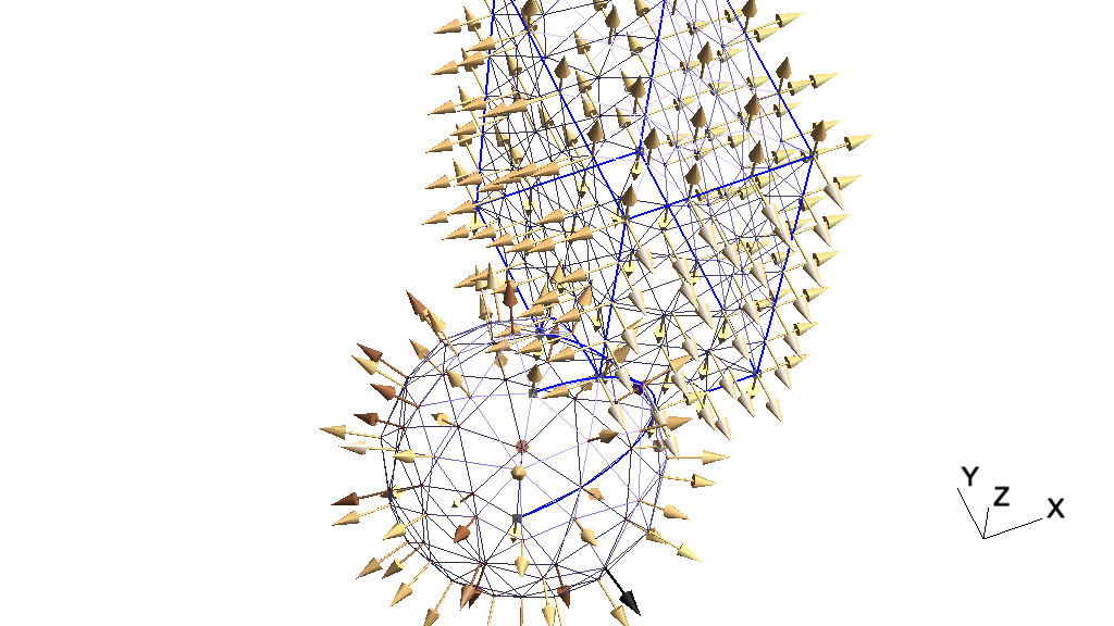
# -----------------------------------------------------------------------------
#
#  Gmsh Python extended tutorial 5
#
#  Additional geometrical data: parametrizations, normals, curvatures
#
# -----------------------------------------------------------------------------

import gmsh
import sys
import math

gmsh.initialize(sys.argv)

# The API provides access to geometrical data in a CAD kernel agnostic manner.

# Let's create a simple CAD model by fusing a sphere and a cube, then mesh the
# surfaces:
gmsh.model.add("x5")
s = gmsh.model.occ.addSphere(0, 0, 0, 1)
b = gmsh.model.occ.addBox(0.5, 0, 0, 1.3, 2, 3)
gmsh.model.occ.fuse([(3, s)], [(3, b)])
gmsh.model.occ.synchronize()
gmsh.model.mesh.generate(2)

# We can for example retrieve the exact normals and the curvature at all the
# mesh nodes (i.e. not normals and curvatures computed from the mesh, but
# directly evaluated on the geometry), by querying the CAD kernels at the
# corresponding parametric coordinates.
normals = []
curvatures = []

# For each surface in the model:
for e in gmsh.model.getEntities(2):
    # Retrieve the surface tag
    s = e[1]

    # Get the mesh nodes on the surface, including those on the boundary
    # (contrary to internal nodes, which store their parametric coordinates,
    # boundary nodes will be reparametrized on the surface in order to compute
    # their parametric coordinates, the result being different when
    # reparametrized on another adjacent surface)
    tags, coord, param = gmsh.model.mesh.getNodes(2, s, True)

    # Get the surface normals on all the points on the surface corresponding to
    # the parametric coordinates of the nodes
    norm = gmsh.model.getNormal(s, param)

    # In the same way, get the curvature
    curv = gmsh.model.getCurvature(2, s, param)

    # Store the normals and the curvatures so that we can display them as
    # list-based post-processing views
    for i in range(0, len(coord), 3):
        normals.append(coord[i])
        normals.append(coord[i + 1])
        normals.append(coord[i + 2])
        normals.append(norm[i])
        normals.append(norm[i + 1])
        normals.append(norm[i + 2])
        curvatures.append(coord[i])
        curvatures.append(coord[i + 1])
        curvatures.append(coord[i + 2])
        curvatures.append(curv[i // 3])

# Create a list-based vector view on points to display the normals, and a scalar
# view on points to display the curvatures
vn = gmsh.view.add("normals")
gmsh.view.addListData(vn, "VP", len(normals) // 6, normals)
gmsh.view.option.setNumber(vn, 'ShowScale', 0)
gmsh.view.option.setNumber(vn, 'ArrowSizeMax', 30)
gmsh.view.option.setNumber(vn, 'ColormapNumber', 19)
vc = gmsh.view.add("curvatures")
gmsh.view.addListData(vc, "SP", len(curvatures) // 4, curvatures)
gmsh.view.option.setNumber(vc, 'ShowScale', 0)

# We can also retrieve the parametrization bounds of model entities, e.g. of
# curve 5, and evaluate the parametrization for several parameter values:
bounds = gmsh.model.getParametrizationBounds(1, 5)
N = 20
t = [bounds[0][0] + i * (bounds[1][0] - bounds[0][0]) / N for i in range(N)]
xyz1 = gmsh.model.getValue(1, 5, t)

# We can also reparametrize curve 5 on surface 1, and evaluate the points in the
# parametric plane of the surface:
uv = gmsh.model.reparametrizeOnSurface(1, 5, t, 1)
xyz2 = gmsh.model.getValue(2, 1, uv)

# Hopefully we get the same x, y, z coordinates!
if max([abs(a - b) for (a, b) in zip(xyz1, xyz2)]) < 1e-12:
    gmsh.logger.write('Evaluation on curve and surface match!')
else:
    gmsh.logger.write('Evaluation on curve and surface do not match!', 'error')

# Launch the GUI to see the results:
if '-nopopup' not in sys.argv:
    gmsh.fltk.run()

gmsh.finalize()
2.27 x6: Additional mesh data: integration points, Jacobians and basis functions 
See x6.py. Also available in C++ (x6.cpp) and Julia (x6.jl).
# -----------------------------------------------------------------------------
#
#  Gmsh Python extended tutorial 6
#
#  Additional mesh data: integration points, Jacobians and basis functions
#
# -----------------------------------------------------------------------------

import gmsh
import sys

gmsh.initialize(sys.argv)

gmsh.model.add("x6")

# The API provides access to all the elementary building blocks required to
# implement finite-element-type numerical methods. Let's create a simple 2D
# model and mesh it:
gmsh.model.occ.addRectangle(0, 0, 0, 1, 0.1)
gmsh.model.occ.synchronize()
gmsh.model.mesh.setTransfiniteAutomatic()
gmsh.model.mesh.generate(2)

# Set the element order and the desired interpolation order:
elementOrder = 1
interpolationOrder = 2
gmsh.model.mesh.setOrder(elementOrder)

def pp(label, v, mult):
    print(" * " + str(len(v) / mult) + " " + label + ": " + str(v))

# Iterate over all the element types present in the mesh:
elementTypes = gmsh.model.mesh.getElementTypes()

for t in elementTypes:
    # Retrieve properties for the given element type
    elementName, dim, order, numNodes, localNodeCoord, numPrimNodes =\
    gmsh.model.mesh.getElementProperties(t)
    print("\n** " + elementName + " **\n")

    # Retrieve integration points for that element type, enabling exact
    # integration of polynomials of order "interpolationOrder". The "Gauss"
    # integration family returns the "economical" Gauss points if available, and
    # defaults to the "CompositeGauss" (tensor product) rule if not.
    localCoords, weights =\
    gmsh.model.mesh.getIntegrationPoints(t, "Gauss" + str(interpolationOrder))
    pp("integration points to integrate order " +
       str(interpolationOrder) + " polynomials", localCoords, 3)

    # Return the basis functions evaluated at the integration points. Selecting
    # "Lagrange" and "GradLagrange" returns the isoparamtric basis functions and
    # their gradient (in the reference space of the given element type). A
    # specific interpolation order can be requested using "LagrangeN" and
    # "GradLagrangeN" with N = 1, 2, ... Other supported function spaces include
    # "H1LegendreN", "GradH1LegendreN", "HcurlLegendreN", "CurlHcurlLegendreN".
    numComponents, basisFunctions, numOrientations =\
    gmsh.model.mesh.getBasisFunctions(t, localCoords, "Lagrange")
    pp("basis functions at integration points", basisFunctions, 1)
    numComponents, basisFunctions, numOrientations =\
    gmsh.model.mesh.getBasisFunctions(t, localCoords, "GradLagrange")
    pp("basis function gradients at integration points", basisFunctions, 3)

    # Compute the Jacobians (and their determinants) at the integration points
    # for all the elements of the given type in the mesh. Beware that the
    # Jacobians are returned "by column": see the API documentation for details.
    jacobians, determinants, coords =\
    gmsh.model.mesh.getJacobians(t, localCoords)
    pp("Jacobian determinants at integration points", determinants, 1)

gmsh.finalize()
2.28 x7: Additional mesh data: internal edges and faces 
See x7.py. Also available in C++ (x7.cpp) and Julia (x7.jl).
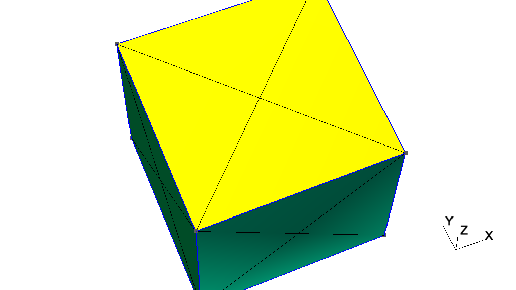
# -----------------------------------------------------------------------------
#
#  Gmsh Python extended tutorial 7
#
#  Additional mesh data: internal edges and faces
#
# -----------------------------------------------------------------------------

import sys
import gmsh

gmsh.initialize(sys.argv)

gmsh.model.add("x7")

# Meshes are fully described in Gmsh by nodes and elements, both associated to
# model entities. The API can be used to generate and handle other mesh
# entities, i.e. mesh edges and faces, which are not stored by default.

# Let's create a simple model and mesh it:
gmsh.model.occ.addBox(0, 0, 0, 1, 1, 1)
gmsh.model.occ.synchronize()
gmsh.option.setNumber("Mesh.MeshSizeMin", 2.)
gmsh.model.mesh.generate(3)

# Like elements, mesh edges and faces are described by (an ordered list of)
# their nodes. Let us retrieve the edges and the (triangular) faces of all the
# first order tetrahedra in the mesh:
elementType = gmsh.model.mesh.getElementType("tetrahedron", 1)
edgeNodes = gmsh.model.mesh.getElementEdgeNodes(elementType)
faceNodes = gmsh.model.mesh.getElementFaceNodes(elementType, 3)

# Edges and faces are returned for each element as a list of nodes corresponding
# to the canonical orientation of the edges and faces for a given element type.

# Gmsh can also identify unique edges and faces (a single edge or face whatever
# the ordering of their nodes) and assign them a unique tag. This identification
# can be done internally by Gmsh (e.g. when generating keys for basis
# functions), or requested explicitly as follows:
gmsh.model.mesh.createEdges()
gmsh.model.mesh.createFaces()

# Edge and face tags can then be retrieved by providing their nodes:
edgeTags, edgeOrientations = gmsh.model.mesh.getEdges(edgeNodes)
faceTags, faceOrientations = gmsh.model.mesh.getFaces(3, faceNodes)

# Since element edge and face nodes are returned in the same order as the
# elements, one can easily keep track of which element(s) each edge or face is
# connected to:
elementTags, elementNodeTags = gmsh.model.mesh.getElementsByType(elementType)
edges2Elements = {}
faces2Elements = {}
for i in range(len(edgeTags)): # 6 edges per tetrahedron
    if not edgeTags[i] in edges2Elements:
        edges2Elements[edgeTags[i]] = [elementTags[i // 6]]
    else:
        edges2Elements[edgeTags[i]].append(elementTags[i // 6])
for i in range(len(faceTags)): # 4 faces per tetrahedron
    if not faceTags[i] in faces2Elements:
        faces2Elements[faceTags[i]] = [elementTags[i // 4]]
    else:
        faces2Elements[faceTags[i]].append(elementTags[i // 4])

# New unique lower dimensional elements can also be easily created given the
# edge or face nodes. This is especially useful for numerical methods that
# require integrating or interpolating on internal edges or faces (like
# e.g. Discontinuous Galerkin techniques), since creating elements for the
# internal entities will make this additional mesh data readily available (see
# `x6.py'). For example, we can create a new discrete surface...
s = gmsh.model.addDiscreteEntity(2)

# ... and fill it with unique triangles corresponding to the faces of the
# tetrahedra:
maxElementTag = gmsh.model.mesh.getMaxElementTag()
uniqueFaceTags = set()
tagsForTriangles = []
faceNodesForTriangles = []
for i in range(len(faceTags)):
    if faceTags[i] not in uniqueFaceTags:
        uniqueFaceTags.add(faceTags[i])
        tagsForTriangles.append(faceTags[i] + maxElementTag)
        faceNodesForTriangles.append(faceNodes[3 * i])
        faceNodesForTriangles.append(faceNodes[3 * i + 1])
        faceNodesForTriangles.append(faceNodes[3 * i + 2])
elementType2D = gmsh.model.mesh.getElementType("triangle", 1)
gmsh.model.mesh.addElementsByType(s, elementType2D, tagsForTriangles,
                                  faceNodesForTriangles)

# Since the tags for the triangles have been created based on the face tags,
# the information about neighboring elements can also be readily created,
# useful e.g. in Finite Volume or Discontinuous Galerkin techniques:
for t in tagsForTriangles:
    print("triangle " + str(int(t)) + " is connected to tetrahedra " +
          str(faces2Elements[t - maxElementTag]))

# If all you need is the list of all edges or faces in terms of their nodes, you
# can also directly call:
edgeTags, edgeNodes = gmsh.model.mesh.getAllEdges()
faceTags, faceNodes = gmsh.model.mesh.getAllFaces(3)

# Launch the GUI to see the results:
if '-nopopup' not in sys.argv:
    gmsh.fltk.run()

gmsh.finalize()
3 Gmsh graphical user interface 
Once you have the Gmsh application installed (see Installing and running Gmsh on your computer), to launch the graphical interface just double-click on the Gmsh icon, or type
> gmsh
at the shell prompt in a terminal. This will open the main window of the
Gmsh GUI, with a menu bar on top (except on macOS, where by default the
menu bar is on the top of the screen – this can be changed with the
General.SystemMenuBar option, see General options), a tree
menu on the left (which by default contains a ‘Modules’ entry with three
children: ‘Geometry’, ‘Mesh’ and ‘Solver’), a graphic area on the right,
and a status bar with some shortcut buttons at the bottom. (You can
detach the tree menu using ‘Window->Attach/Detach Menu’.)
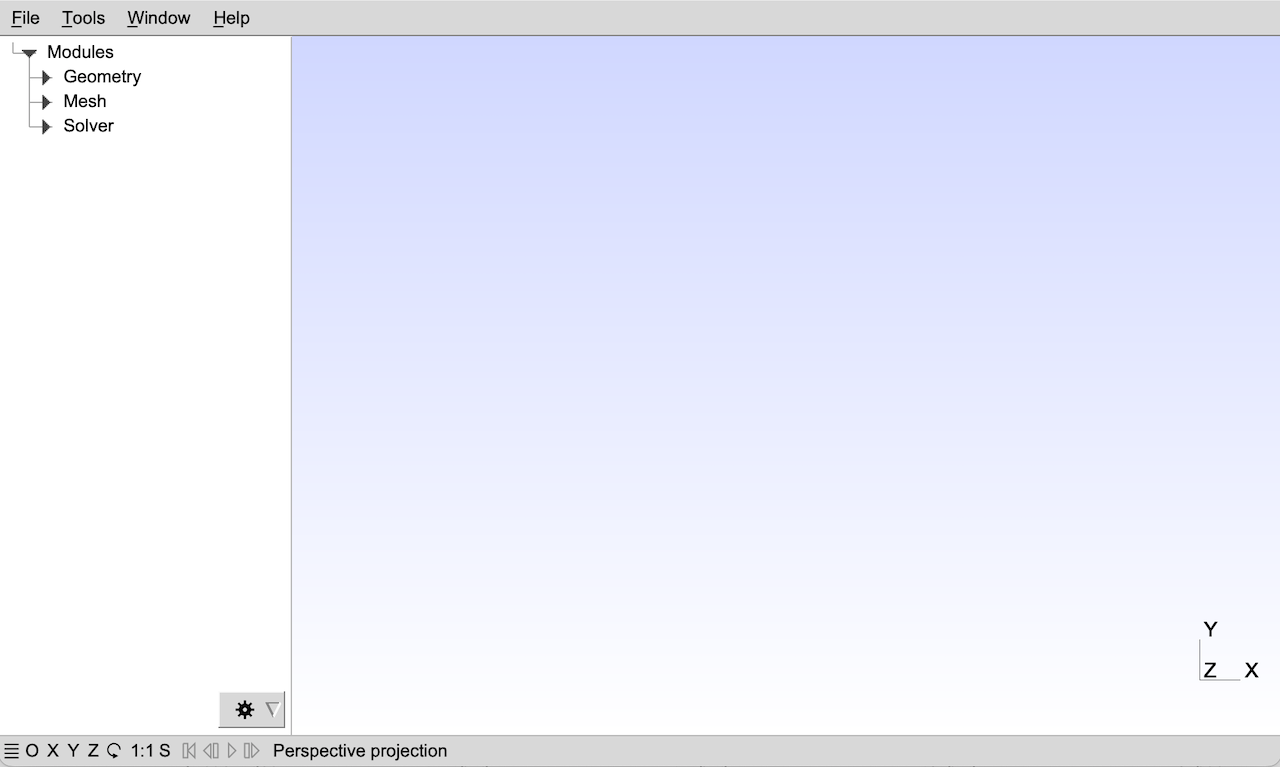
To create a new geometrical model, use the ‘File->New’ menu to create a new model file, and choose for example mymodel.geo as file name. Then in the tree menu, successively open the ‘Geometry’, ‘Elementary entities’ and ‘Add’ submenus, and click for example on ‘Rectangle’. A context window with parameters will pop up: you can enter some parameters in this window (e.g. the width and height of the rectangle) and move the mouse to place it on the canvas. If you don’t want to place the rectangle with the mouse, select ‘X’, ‘Y’ and ‘Z freeze’ in the window and enter the coordinates manually in the context window. Once you are done, either press e (see the status message on the top of the graphic window) or click on the ‘Add’ button in the context window.
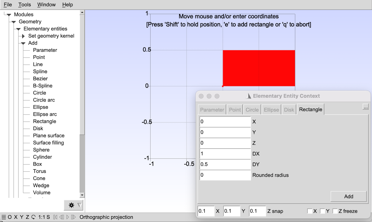
There is no need to save your geometrical model: when the rectangle was added, scripting commands were automatically appended to your model file mymodel.geo:
//+
SetFactory("OpenCASCADE");
Rectangle(1) = {0, 0, 0, 1, 0.5, 0};
You can edit this script with any text editor; clicking on ‘Edit script’
in the tree menu will launch the default text editor specified by the
General.Editor option (see General options). If you edit the
script, you should click on ‘Reload script’ in the tree menu to reload
the modifications in the GUI. The //+ line in the script is a
comment that is used as a placemark between commands added by the GUI;
see Gmsh scripting language for the scripting language reference.
Combining GUI actions and script file editing is a classical way of working with the Gmsh app. For example, it is often faster to define variables and points directly in the script file, and then use the GUI to define the curves, the surfaces and the volumes interactively.
To load an existing model instead of creating a model from scratch, use the ‘File->Open’ menu. For example, to open the first tutorial (see Gmsh tutorial), choose t1.geo. On the terminal, you can also specify the file name directly on the command line, i.e.:
> gmsh t1.geo
To generate a mesh, open ‘Mesh’ in the tree menu and choose the desired dimension: ‘1D’ will mesh all the curves; ‘2D’ will mesh all the surfaces—as well as all the curves if ‘1D’ was not called before; ‘3D’ will mesh all the volumes—and all the surfaces if ‘2D’ was not called before. To save the resulting mesh in the current mesh format click on ‘Save’ in the tree menu, or select the appropriate format and file name with the ‘File->Export’ menu. The default mesh file name is based on the name of the current active model, with an appended extension depending on the mesh format. Note that most interactive commands have keyboard shortcuts: see Keyboard shortcuts, or select ‘Help->Keyboard and Mouse Usage’ in the menu. For example, to quickly generate the 2D mesh and save a mesh, you can first press 2, then Ctrl+Shift+s.
A double-click in the graphic window will pop up a quick shortcut menu, which can be used e.g. to quickly toggle the visibility of mesh entities (like surface faces), reset the viewport, select the rotation center, display axes, or access the full module options (from the ‘Tools->Options’ menu). The shortcut buttons on the bottom left of the status bar can be used to quickly adjust the viewport: ‘X’, ‘Y’, ‘Z’ set viewports with the corresponding axis perpendicular to graphic plane; the rotation button rotates the view by 90 degrees; and ‘1:1’ resets the scale.
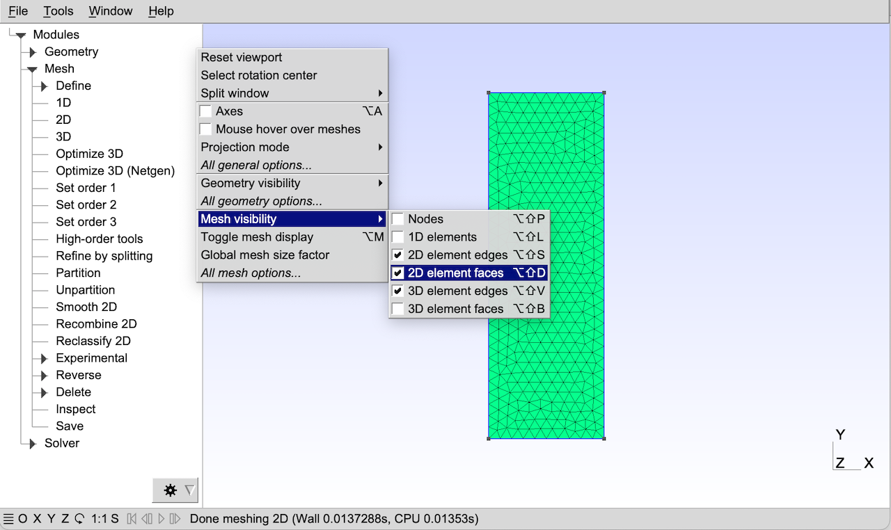
Several files can be loaded simultaneously. When specified on the
command line, the first one defines the active model (in the same way as
using the ‘File->Open’ menu) and the others are ‘merged’ into this model
(in the same way as using the the ‘File->Merge’ menu). For example, to
merge the post-processing views contained in the files
view1.pos and
view5.msh together with
the geometry of the first tutorial t1: Geometry basics, elementary entities, physical groups, you can type the following
command:
> gmsh t1.geo view1.pos view5.msh
When one or more more post-processing views are loaded, a ‘Post-Processing’ entry in the tree menu appears. With the previous command, three views will appear in the tree menu under ‘Post-processing’, respectively labeled ‘A scalar map’, ‘Nodal scalar map’ and ‘Element 1 vector’. In this example the views contain several time steps: you can loop through them with the shortcuts icons on the left of the status bar. A mouse click on the view name will toggle the visibility of the selected view, while a click on the arrow button on the right will provide access to the view’s options.
Note that all the options specified interactively can also be directly specified in the script files. You can save the current options of the current active model with the ‘File->Save Model Options’. This will create a new option file with the same filename as the active model, but with an extra .opt extension added. The next time you open this model, the associated options will be automatically loaded, too. To save the current options as your default preferences for all future Gmsh sessions, use the ‘File->Save Options As Default’ menu instead. You can also save the current options in an arbitrary file by choosing the ‘Gmsh options’ format in ‘File->Export’. For more information about available options (and how to reset them to their default values), see Gmsh options. A full list of options with their current values is also available using the ‘Help->Current Options’ menu.
Finally, note that the GUI can also be run (and modified) using the API:
see Namespace gmsh/fltk: FLTK graphical user interface functions for details.
The two next sections describe the mouse actions in the GUI, as well as all the predefined keyboard shortcuts. Screencasts explaining how to use the Gmsh GUI are available online at the following address: https://gmsh.info/screencasts/.
3.1 Mouse actions 
- Move
Highlight the entity under the mouse pointer and display its properties / Resize a lasso zoom or a lasso (un)selection
- Left button
Rotate / Select an entity / Accept a lasso zoom or a lasso selection
- Ctrl+Left button
Start a lasso zoom or a lasso (un)selection
- Middle button
Zoom / Unselect an entity / Accept a lasso zoom or a lasso unselection
- Ctrl+Middle button
Orthogonalize display
- Right button
Pan / Cancel a lasso zoom or a lasso (un)selection / Pop-up menu on post-processing view button
- Ctrl+Right button
Reset to default viewpoint
For a 2 button mouse, Middle button = Shift+Left button.
For a 1 button mouse, Middle button = Shift+Left button, Right button = Alt+Left button.
3.2 Keyboard shortcuts 
(On macOS, Ctrl is replaced by Cmd in the shortcuts below.)
- Left arrow
Go to previous time step
- Right arrow
Go to next time step
- Up arrow
Make previous view visible
- Down arrow
Make next view visible
- 0
Reload geometry
- Ctrl+0 or 9
Reload full project
- 1 or F1
Mesh lines
- 2 or F2
Mesh surfaces
- 3 or F3
Mesh volumes
- Escape
Cancel lasso zoom/selection, toggle mouse selection ON/OFF
- e
End/accept selection in geometry creation mode
- g
Go to geometry module
- m
Go to mesh module
- p
Go to post-processing module
- q
Abort selection in geometry creation mode
- s
Go to solver module
- x
Toggle x coordinate freeze in geometry creation mode
- y
Toggle y coordinate freeze in geometry creation mode
- z
Toggle z coordinate freeze in geometry creation mode
- Shift+a
Bring all windows to front
- Shift+g
Show geometry options
- Shift+m
Show mesh options
- Shift+o
Show general options
- Shift+p
Show post-processing options
- Shift+s
Show solver options
- Shift+u
Show post-processing view plugins
- Shift+w
Show post-processing view options
- Shift+x
Move only along x coordinate in geometry creation mode
- Shift+y
Move only along y coordinate in geometry creation mode
- Shift+z
Move only along z coordinate in geometry creation mode
- Shift+Escape
Enable full mouse selection
- Ctrl+d
Attach/detach menu
- Ctrl+e
Export project
- Ctrl+f
Enter full screen
- Ctrl+i
Show statistics window
- Ctrl+j
Save model options
- Ctrl+l
Show message console
- Ctrl+m
Minimize window
- Ctrl+n
Create new project file
- Ctrl+o
Open project file
- Ctrl+q
Quit
- Ctrl+r
Rename project file
- Ctrl+s
Save mesh in default format
- Shift+Ctrl+c
Show clipping plane window
- Shift+Ctrl+h
Show current options and workspace window
- Shift+Ctrl+j
Save options as default
- Shift+Ctrl+m
Show manipulator window
- Shift+Ctrl+n
Show option window
- Shift+Ctrl+o
Merge file(s)
- Shift+Ctrl+r
Open next-to-last opened file
- Shift+Ctrl+u
Show plugin window
- Shift+Ctrl+v
Show visibility window
- Alt+a
Loop through axes modes
- Alt+b
Hide/show bounding boxes
- Alt+c
Loop through predefined color schemes
- Alt+e
Hide/Show element outlines for visible post-pro views
- Alt+f
Change redraw mode (fast/full)
- Alt+h
Hide/show all post-processing views
- Alt+i
Hide/show all post-processing view scales
- Alt+l
Hide/show geometry lines
- Alt+m
Toggle visibility of all mesh entities
- Alt+n
Hide/show all post-processing view annotations
- Alt+o
Change projection mode (orthographic/perspective)
- Alt+p
Hide/show geometry points
- Alt+r
Loop through range modes for visible post-pro views
- Alt+s
Hide/show geometry surfaces
- Alt+t
Loop through interval modes for visible post-pro views
- Alt+v
Hide/show geometry volumes
- Alt+w
Enable/disable all lighting
- Alt+x
Set X view
- Alt+y
Set Y view
- Alt+z
Set Z view
- Alt+1
Set 1:1 view
- Alt+Shift+a
Hide/show small axes
- Alt+Shift+b
Hide/show mesh volume faces
- Alt+Shift+c
Loop through predefined colormaps
- Alt+Shift+d
Hide/show mesh surface faces
- Alt+Shift+l
Hide/show mesh lines
- Alt+Shift+p
Hide/show mesh nodes
- Alt+Shift+s
Hide/show mesh surface edges
- Alt+Shift+t
Same as Alt+t, but with numeric mode included
- Alt+Shift+v
Hide/show mesh volume edges
- Alt+Shift+x
Set -X view
- Alt+Shift+y
Set -Y view
- Alt+Shift+z
Set -Z view
- Alt+Shift+1
Reset bounding box around visible entities
- Alt+Ctrl++1
Sync scale between viewports
4 Gmsh command-line interface 
Gmsh defines a number of commands-line switches that can be used to control Gmsh in “batch” mode from the command line, and pass options without resorting to a script (see Gmsh scripting language) or the API (see Gmsh application programming interface).
For example, meshing the first tutorial in batch mode can be done in a
terminal by passing the -2 command-line switch:
> gmsh t1.geo -2
The same effect could be achieved by adding the Mesh 2; command
at the end of t1.geo and running
> gmsh t1.geo -parse_and_exit
or further adding the Exit; command at the end of the script and
simply opening this new file:
> gmsh t1.geo
Note that all numeric and string options (see Gmsh options) can be
set from the command line with the -setnumber and
-setstring switches
> gmsh t1.geo -setnumber Mesh.Nodes 1 -setnumber Geometry.SurfaceLabels 1
The list of all command-line switches is given hereafter.
(Related option names, if any, are given between parentheses)
Geometry:
-0¶Output model, then exit
-tol value¶Set geometrical tolerance (Geometry.Tolerance)
-match¶Match geometries and meshes
Mesh:
-1, -2, -3¶Perform 1D, 2D or 3D mesh generation, then exit
-format string¶Select output mesh format: auto, msh1, msh2, msh22, msh3, msh4, msh40, msh41, msh, unv, vtk, wrl, mail, stl, p3d, mesh, bdf, cgns, med, diff, ir3, inp, ply2, celum, su2, x3d, dat, neu, m, key, off, rad, obj (Mesh.Format)
-bin¶Create binary files when possible (Mesh.Binary)
-refine¶Perform uniform mesh refinement, then exit
-barycentric_refine¶Perform barycentric mesh refinement, then exit
-reclassify angle¶Reclassify surface mesh, then exit
-reparam angle¶Reparametrize surface mesh, then exit
-hybrid¶generate a hybrid hex-tet mesh with trihedron for transitions
-part int¶Partition after batch mesh generation (Mesh.NbPartitions)
-part_weight [tri,quad,tet,hex,pri,pyr,trih] int¶Weight of a triangle/quad/etc. during partitioning (Mesh.Partition[Tri,Quad,...]Weight)
-part_split¶Save mesh partitions in separate files (Mesh.PartitionSplitMeshFiles)
-part_[no_]topo¶Create the partition topology (Mesh.PartitionCreateTopology)
-part_[no_]ghosts¶Create ghost cells (Mesh.PartitionCreateGhostCells)
-part_[no_]physicals¶Create physical groups for partitions (Mesh.PartitionCreatePhysicals)
-part_topo_pro¶Save the partition topology .pro file (Mesh.PartitionTopologyFile)
-overlap int¶Create partition overlaps after batch mesh generation (Mesh.OverlapLayers)
-preserve_numbering_msh2¶Preserve element numbering in MSH2 format (Mesh.PreserveNumberingMsh2)
-save_all¶Save all elements (Mesh.SaveAll)
-save_parametric¶Save nodes with their parametric coordinates (Mesh.SaveParametric)
-save_topology¶Save model topology (Mesh.SaveTopology)
-algo string¶Select mesh algorithm: auto, meshadapt, del2d, front2d, delquad, quadqs, initial2d, del3d, front3d, mmg3d, hxt, initial3d (Mesh.Algorithm and Mesh.Algorithm3D)
-smooth int¶Set number of mesh smoothing steps (Mesh.Smoothing)
-order int¶Set mesh order (Mesh.ElementOrder)
-optimize[_netgen]¶Optimize quality of tetrahedral elements (Mesh.Optimize[Netgen])
-optimize_threshold¶Optimize tetrahedral elements that have a quality less than a threshold (Mesh.OptimizeThreshold)
-optimize_ho¶Optimize high order meshes (Mesh.HighOrderOptimize)
-ho_[min,max,nlayers]¶High-order optimization parameters (Mesh.HighOrderThreshold[Min,Max], Mesh.HighOrderNumLayers)
-clscale value¶Set mesh element size factor (Mesh.MeshSizeFactor)
-clmin value¶Set minimum mesh element size (Mesh.MeshSizeMin)
-clmax value¶Set maximum mesh element size (Mesh.MeshSizeMax)
-clextend value¶Extend mesh element sizes from boundaries (Mesh.MeshSizeExtendFromBoundary)
-clcurv value¶Compute mesh element size from curvature, with value the target number of elements per 2*pi radians (Mesh.MeshSizeFromCurvature)
-aniso_max value¶Set maximum anisotropy for bamg (Mesh.AnisoMax)
-smooth_ratio value¶Set smoothing ration between mesh sizes at nodes of a same edge for bamg (Mesh.SmoothRatio)
-epslc1d value¶Set accuracy of evaluation of mesh size field for 1D mesh (Mesh.LcIntegrationPrecision)
-swapangle value¶Set the threshold angle (in degrees) between two adjacent faces below which a swap is allowed (Mesh.AllowSwapAngle)
-rand value¶Set random perturbation factor (Mesh.RandomFactor)
-bgm file¶Load background mesh from file
-check¶Perform various consistency checks on mesh
-ignore_periocity¶Ignore periodic boundaries (Mesh.IgnorePeriodicity)
Post-processing:
-link int¶Select link mode between views (PostProcessing.Link)
-combine¶Combine views having identical names into multi-time-step views
Solver:
-listen string¶Always listen to incoming connection requests (Solver.AlwaysListen) on the given socket (uses Solver.SocketName if not specified)
-minterpreter string¶Name of Octave interpreter (Solver.OctaveInterpreter)
-pyinterpreter string¶Name of Python interpreter (Solver.OctaveInterpreter)
-run¶Run ONELAB solver(s)
Display:
-n¶Hide all meshes and post-processing views on startup (View.Visible, Mesh.[Points,Lines,SurfaceEdges,...])
-nodb¶Disable double buffering (General.DoubleBuffer)
-numsubedges¶Set num of subdivisions for high order element display (Mesh.NumSubEdges)
-fontsize int¶Specify the font size for the GUI (General.FontSize)
-theme string¶Specify FLTK GUI theme (General.FltkTheme)
-display string¶Specify display (General.Display)
-camera¶Use camera mode view (General.CameraMode)
-stereo¶OpenGL quad-buffered stereo rendering (General.Stereo)
-gamepad¶Use gamepad controller if available
Other:
-, -parse_and_exit¶Parse input files, then exit
-save¶Save output file, then exit
-o file¶Specify output file name
-new¶Create new model before merge next file
-merge¶Merge next files
-open¶Open next files
-log filename¶Log all messages to filename
-a, -g, -m, -s, -p¶Start in automatic, geometry, mesh, solver or post-processing mode (General.InitialModule)
-pid¶Print process id on stdout
-watch pattern¶Pattern of files to merge as they become available (General.WatchFilePattern)
-bg file¶Load background (image or PDF) file (General.BackgroundImageFileName)
-v int¶Set verbosity level (General.Verbosity)
-string "string"¶Parse command string at startup
-setnumber name value¶Set constant, ONELAB or option number name=value
-setstring name value¶Set constant, ONELAB or option string name=value
-nopopup¶Don’t popup dialog windows in scripts (General.NoPopup)
-noenv¶Don’t modify the environment at startup
-nolocale¶Don’t modify the locale at startup
-option file¶Parse option file at startup
-convert files¶Convert files into latest binary formats, then exit
-nt int¶Set number of threads (General.NumThreads)
-cpu¶Report CPU times for all operations
-version¶Show version number
-info¶Show detailed version information
-help¶Show command line usage
-help_options¶Show all options
5 Gmsh scripting language 
The Gmsh scripting language is interpreted at runtime by Gmsh’s parser. Scripts are written in ASCII files and are usually given the .geo extension, but any extension (or no extension at all) can also be used. For example Gmsh often uses the .pos extension for scripts that contain post-processing commands, in particular parsed post-processing views (see Post-processing scripting commands).
Historically, .geo scripts have been the primary way to perform complex tasks with Gmsh, and they are indeed quite powerful: they can handle (lists of) floating point (see Floating point expressions) and string (see String expressions) variables, loops and tests (see Loops and conditionals), macros (see User-defined macros), etc. However Gmsh’s scripting language is still quite limited compared to actual programming languages: for example there are no private variables, macros don’t take arguments, and the runtime interpretation by the parser can penalize performance on large models. Depending on the workflow and the application, using the Gmsh API (see Gmsh application programming interface) can thus sometimes be preferable. The downside of the API is that, while the scripting language is baked into Gmsh and is thus available directly in the standalone Gmsh app, the API requires external dependencies (a C++, C or Fortran compiler; or a Python or Julia interpreter).
This chapter describes the scripting language by detailing general commands first (see General scripting commands), before detailing the scripting commands specific to the geometry (see Geometry scripting commands), mesh (see Mesh scripting commands) and post-processing (see Post-processing scripting commands) modules.
The following rules are used when describing the scripting language in the rest of this chapter (note that metasyntactic variable definitions stay valid throughout the chapter, not only in the section where the definitions appear):
- Keywords and literal symbols are printed like
this. - Metasyntactic variables (i.e., text bits that are not part of the syntax, but stand for other text bits) are printed like this.
- A colon (
:) after a metasyntactic variable separates the variable from its definition. - Optional rules are enclosed in
<>pairs. - Multiple choices are separated by
|. - Three dots (…) indicate a possible (multiple) repetition of the preceding rule.
In most commands that apply to geometrical entities of several
dimensions with the same syntax (e.g. the creation of Physical
Point | Curve | Surface | Volume), the Point, Curve,
Surface and Volume keywords can be replaced by
GeoEntity { expression }, with expression
respectively equal to 0, 1, 2, or 3. This makes it easier to script
parametric geometries that are valid in several dimensions, without code
duplication.
- General scripting commands
- Geometry scripting commands
- Mesh scripting commands
- Post-processing scripting commands
5.1 General scripting commands 
- Comments
- Floating point expressions
- String expressions
- Color expressions
- Operators
- Built-in functions
- User-defined macros
- Loops and conditionals
- Other general commands
5.1.1 Comments 
Gmsh script files support both C and C++ style comments:
- any text comprised between
/*and*/pairs is ignored; - the rest of a line after a double slash
//is ignored.
These commands won’t have the described effects inside double quotes or inside keywords. Also note that ‘white space’ (spaces, tabs, new line characters) is ignored inside all expressions.
5.1.2 Floating point expressions 
The two constant types used in Gmsh scripts are real and string (there is no integer type). These types have the same meaning and syntax as in the C or C++ programming languages.
Floating point expressions (or, more simply, “expressions”) are denoted by the metasyntactic variable expression, and are evaluated during the parsing of the script file:
expression:
  real |
  string |
  string ~ { expression }
  string [ expression ] |
  # string [ ] |
  ( expression ) |
  operator-unary-left expression |
  expression operator-unary-right |
  expression operator-binary expression |
  expression operator-ternary-left expression
    operator-ternary-right expression |
  built-in-function |
  number-option |
  Find(expression-list-item, expression-list-item) |
  StrFind(string-expression, string-expression) |
  StrCmp(string-expression, string-expression) |
  StrLen(string-expression) |
  TextAttributes(string-expression<,string-expression...>) |
  Exists(string) | Exists(string~{ expression }) |
  FileExists(string-expression) |
  StringToName(string-expression) | S2N(string-expression) |
  GetNumber(string-expression <,expression>) |
  GetValue("string", expression) |
  DefineNumber(expression, onelab-options)
Such expressions are used in most of Gmsh’s scripting
commands. When ~{expression} is appended to a string
string, the result is a new string formed by the concatenation of
string, _ (an underscore) and the value of the
expression. This is most useful in loops (see Loops and conditionals), where it permits to define unique strings
automatically. For example,
For i In {1:3}
  x~{i} = i;
EndFor
is the same as
x_1 = 1;
x_2 = 2;
x_3 = 3;
The brackets [] permit to extract one item from a list
(parentheses can also be used instead of brackets). The # permits
to get the size of a list. The operators operator-unary-left,
operator-unary-right, operator-binary,
operator-ternary-left and operator-ternary-right are defined
in Operators. For the definition of built-in-functions,
see Built-in functions. The various number-options are
listed in Gmsh options. Find searches for occurrences of
the first expression in the second (both of which can be lists).
StrFind searches the first string-expression for any
occurrence of the second string-expression. StrCmp compares
the two strings (returns an integer greater than, equal to, or less than
0, according as the first string is greater than, equal to, or less than
the second string). StrLen returns the length of the
string. TextAttributes creates attributes for text
strings. Exists checks if a variable with the given name exists
(i.e., has been defined previously), and FileExists checks if the
file with the given name exists. StringToName creates a name
from the provided string. GetNumber allows to get the value of a
ONELAB variable (the optional second argument is the default value
returned if the variable does not exist). GetValue allows to ask
the user for a value interactively (the second argument is the value
returned in non-interactive mode). For example, inserting
GetValue("Value of parameter alpha?", 5.76) in an input file will
query the user for the value of a certain parameter alpha, assuming the
default value is 5.76. If the option General.NoPopup is set
(see General options), no question is asked and the default value is
automatically used.
DefineNumber allows to define a ONELAB variable in-line. The
expression given as the first argument is the default value; this
is followed by the various ONELAB options. See the
ONELAB tutorial wiki for more information.
List of expressions are also widely used, and are defined as:
expression-list:
  expression-list-item <, expression-list-item> ...
with
expression-list-item:
  expression |
  expression : expression |
  expression : expression : expression |
  string [ ] |  string ( ) |
  List [ string ] |
  List [ expression-list-item ] |
  List [ { expression-list } ] |
  Unique [ expression-list-item ] |
  Abs [ expression-list-item ] |
  ListFromFile [ expression-char ] |
  LinSpace[ expression, expression, expression ] |
  LogSpace[ expression, expression, expression ] |
  string [ { expression-list } ] |
  Point { expression } |
  transform |
  extrude |
  boolean |
  Point|Curve|Surface|Volume In BoundingBox { expression-list } |
  BoundingBox Point|Curve|Surface|Volume { expression-list } |
  Parametric BoundingBox Curve|Surface { expression } |
  Parametric Point { expression } In Surface { expression } |
  Normal Surface { expression } Parametric { expression, expression } |
  Curvature Curve { expression } Parametric { expression } |
  Curvature Surface { expression } Parametric { expression, expression } |
  Mass Curve|Surface|Volume { expression } |
  CenterOfMass Curve|Surface|Volume { expression } |
  MatrixOfInertia Curve|Surface|Volume { expression } |
  Point { expression } |
  Physical Point|Curve|Surface|Volume { expression-list } |
  <Physical> Point|Curve|Surface|Volume { : } |
The second case in this last definition permits to create a list
containing the range of numbers comprised between two
expressions, with a unit incrementation step. The third case
also permits to create a list containing the range of numbers comprised
between two expressions, but with a positive or negative
incrementation step equal to the third expression. The fourth,
fifth and sixth cases permit to reference an expression list
(parentheses can also be used instead of brackets). Unique sorts
the entries in the list and removes all duplicates. Abs takes
the absolute value of all entries in the list. ListFromFile reads
a list of numbers from a file. LinSpace and LogSpace
construct lists using linear or logarithmic spacing. The next two cases
permit to reference an expression sublist (whose elements are those
corresponding to the indices provided by the expression-list).
The next cases permit to retrieve the indices of entities created
through geometrical transformations, extrusions and boolean operations
(see Transformations, Extrusions and Boolean operations).
The next two cases allow to retrieve entities in a given bounding box,
or get the bounding box of a given entity, with the bounding box
specified as (X min, Y min, Z min, X max, Y max, Z max). Beware that the
order of coordinates is different than in the BoundingBox command
for the scene: see Other general commands. Parametric
BoundingBox retrieves the parametric bounds (U min, U max) and (U min,
V min, U max, V max) or a curve or a surface,
respectively. Parametric Point retrieves the parametric
coordinates U, V of a point on a surface. Normal Surface returns
the normal to a surface evaluated at the specified parametric
coordinates. Curvature Curve and. Curvature Surface return
the curvature of a curve or a surface at the specified parametric
coordinates.
The last cases permit to retrieve the mass, the center of mass or the matrix of inertia of an entity, the coordinates of a given geometry point (see Points), the elementary entities making up physical groups, and the tags of all (physical or elementary) points, curves, surfaces or volumes in the model. These operations all trigger a synchronization of the CAD model with the internal Gmsh model.
To see the practical use of such expressions, have a look at the first
couple of examples in Gmsh tutorial. Note that, in order to
lighten the syntax, you can omit the braces {} enclosing an
expression-list if this expression-list only contains a
single item. Also note that a braced expression-list can be
preceded by a minus sign in order to change the sign of all the
expression-list-items.
For some commands it makes sense to specify all the possible expressions in a list. This is achieved with expression-list-or-all, defined as:
expression-list-or-all:
  expression-list | :
The meaning of “all” (:) depends on context. For example,
Curve { : } will get the ids of all the existing curves in the
model, while Surface { : } will get the ids of all existing
surfaces.
5.1.3 String expressions 
String expressions are defined as:
string-expression:
  "string" |
  string | string[ expression ] |
  Today | OnelabAction | GmshExecutableName |
  CurrentDirectory | CurrentDir | CurrentFileName
  StrPrefix ( string-expression ) |
  StrRelative ( string-expression ) |
  StrCat ( string-expression <,...> ) |
  Str ( string-expression <,...> ) |
  StrChoice ( expression, string-expression, string-expression ) |
  StrSub( string-expression, expression, expression ) |
  StrSub( string-expression, expression ) |
  UpperCase ( string-expression ) |
  AbsolutePath ( string-expression ) |
  DirName ( string-expression ) |
  Sprintf ( string-expression , expression-list ) |
  Sprintf ( string-expression ) |
  Sprintf ( string-option ) |
  GetEnv ( string-expression ) |
  GetString ( string-expression <,string-expression>) |
  GetStringValue ( string-expression , string-expression ) |
  StrReplace ( string-expression , string-expression , string-expression )
  NameToString ( string ) | N2S ( string ) |
  <Physical> Point|Curve|Surface|Volume { expression } |
  DefineString(string-expression, onelab-options)
Today returns the current date. OnelabAction returns the
current ONELAB action (e.g. check or
compute). GmshExecutableName returns the full path of the
Gmsh executable. CurrentDirectory (or CurrentDir) and
CurrentFileName return the directory and file name of the script
being parsed. StrPrefix and StrRelative take the prefix
(e.g. to remove the extension) or the relative path of a given file
name. StrCat and Str concatenate string expressions
(Str adds a newline character after each string except the last).
StrChoice returns the first or second string-expression
depending on the value of expression. StrSub returns the
portion of the string that starts at the character position given by the
first expression and spans the number of characters given by the
second expression or until the end of the string (whichever comes
first; or always if the second expression is not
provided). UpperCase converts the string-expression to
upper case. AbsolutePath returns the absolute path of a
file. DirName returns the directory of a file. Sprintf is
equivalent to the sprintf C function (where
string-expression is a format string that can contain floating
point formatting characters: %e, %g, etc.) The various
string-options are listed in Gmsh options. GetEnvThe gets the value of an environment variable
from the operating system. GetString allows to get a ONELAB
string value (the second optional argument is the default value returned
if the variable does not exist). GetStringValue asks the user
for a value interactively (the second argument is the value used in
non-interactive mode). StrReplace’s arguments are: input string,
old substring, new substring (brackets can be used instead of
parentheses in Str and Sprintf). Physical Point,
etc., or Point, etc., retrieve the name of the physical or
elementary entity, if any. NameToString converts a variable name
into a string.
DefineString allows to define a ONELAB variable in-line. The
string-expression given as the first argument is the default
value; this is followed by the various ONELAB options. See the
ONELAB tutorial wiki for more information.
String expressions are mostly used to specify non-numeric options and
input/output file names. See t8: Post-processing, image export and animations, for an interesting usage of
string-expressions in an animation script.
List of string expressions are defined as:
string-expression-list:
  string-expression <,...>
5.1.4 Color expressions 
Colors expressions are hybrids between fixed-length braced expression-lists and strings:
color-expression:
  string-expression |
  { expression, expression, expression } |
  { expression, expression, expression, expression } |
  color-option
The first case permits to use the X Windows names to refer to colors,
e.g., Red, SpringGreen, LavenderBlush3, …
(see src/common/Colors.h
in the source code for a complete list). The second case permits to
define colors by using three expressions to specify their red, green and
blue components (with values comprised between 0 and 255). The third
case permits to define colors by using their red, green and blue color
components as well as their alpha channel. The last case permits to use
the value of a color-option as a color-expression. The
various color-options are listed in Gmsh options.
See t3: Extruded meshes, ONELAB parameters, options, for an example of the use of color expressions.
5.1.5 Operators 
Gmsh’s operators are similar to the corresponding operators in C and C++. Here is the list of available unary, binary and ternary operators.
operator-unary-left:
operator-unary-right:
operator-binary:
^¶Exponentiation.
*¶Multiplication.
/¶Division.
%¶Modulo.
+¶Addition.
-¶Subtraction.
==¶Equality.
!=¶Inequality.
>¶Greater.
>=¶Greater or equality.
<¶Less.
<=¶Less or equality.
&&¶Logical ‘and’.
||¶Logical ‘or’. (Warning: the logical ‘or’ always implies the evaluation of both arguments. That is, unlike in C or C++, the second operand of
||is evaluated even if the first one is true).
operator-ternary-left:
?
operator-ternary-right:
:¶The only ternary operator, formed by operator-ternary-left and operator-ternary-right, returns the value of its second argument if the first argument is non-zero; otherwise it returns the value of its third argument.
The evaluation priorities are summarized below12 (from stronger to
weaker, i.e., * has a highest evaluation priority than +).
Parentheses () may be used anywhere to change the order of
evaluation:
-
(),[],.,# -
^ -
!,++,--,-(unary) -
*,/,% -
+,- -
<,>,<=,>= -
==,!= -
&& -
|| -
?: -
=,+=,-=,*=,/=
5.1.6 Built-in functions 
A built-in function is composed of an identifier followed by a pair of parentheses containing an expression-list, the list of its arguments. This list of arguments can also be provided in between brackets, instead of parentheses. Here is the list of the built-in functions currently implemented:
build-in-function:
Acos ( expression )¶Arc cosine (inverse cosine) of an expression in [-1,1]. Returns a value in [0,Pi].
Asin ( expression )¶Arc sine (inverse sine) of an expression in [-1,1]. Returns a value in [-Pi/2,Pi/2].
Atan ( expression )¶Arc tangent (inverse tangent) of expression. Returns a value in [-Pi/2,Pi/2].
Atan2 ( expression, expression )¶Arc tangent (inverse tangent) of the first expression divided by the second. Returns a value in [-Pi,Pi].
Ceil ( expression )¶Rounds expression up to the nearest integer.
Cos ( expression )¶Cosine of expression.
Cosh ( expression )¶Hyperbolic cosine of expression.
Exp ( expression )¶Returns the value of e (the base of natural logarithms) raised to the power of expression.
Fabs ( expression )¶Absolute value of expression.
Fmod ( expression, expression )¶Remainder of the division of the first expression by the second, with the sign of the first.
Floor ( expression )¶Rounds expression down to the nearest integer.
Hypot ( expression, expression )¶Returns the square root of the sum of the square of its two arguments.
Log ( expression )¶Natural logarithm of expression (expression > 0).
Log10 ( expression )¶Base 10 logarithm of expression (expression > 0).
Max ( expression, expression )¶Maximum of the two arguments.
Min ( expression, expression )¶Minimum of the two arguments.
Modulo ( expression, expression )¶see
Fmod( expression, expression ).Rand ( expression )¶Random number between zero and expression.
Round ( expression )¶Rounds expression to the nearest integer.
Sqrt ( expression )¶Square root of expression (expression >= 0).
Sin ( expression )¶Sine of expression.
Sinh ( expression )¶Hyperbolic sine of expression.
Step ( expression )¶Returns 0 if expression is negative, 1 if not.
Tan ( expression )¶Tangent of expression.
Tanh ( expression )¶Hyperbolic tangent of expression.
5.1.7 User-defined macros 
User-defined macros take no arguments, and are evaluated as if a file
containing the macro body was included at the location of the
Call statement.
Macro string | string-expression¶Begin the declaration of a user-defined macro named string. The body of the macro starts on the line after ‘
Macro string’, and can contain any Gmsh command. A synonym forMacroisFunction.Return¶End the body of the current user-defined macro. Macro declarations cannot be imbricated.
Call string | string-expression ;¶Execute the body of a (previously defined) macro named string.
See t5: Mesh sizes, macros, loops, holes in volumes, for an example of a user-defined macro. A
shortcoming of Gmsh’s scripting language is that all variables are
“public”. Variables defined inside the body of a macro will thus be
available outside, too!
5.1.8 Loops and conditionals 
Loops and conditionals are defined as follows, and can be imbricated:
For ( expression : expression )¶Iterate from the value of the first expression to the value of the second expression, with a unit incrementation step. At each iteration, the commands comprised between ‘
For ( expression : expression )’ and the matchingEndForare executed.For ( expression : expression : expression )¶Iterate from the value of the first expression to the value of the second expression, with a positive or negative incrementation step equal to the third expression. At each iteration, the commands comprised between ‘
For ( expression : expression :
expression )
’ and the matchingEndForare executed.For string In { expression : expression }¶Iterate from the value of the first expression to the value of the second expression, with a unit incrementation step. At each iteration, the value of the iterate is affected to an expression named string, and the commands comprised between ‘
For string
In { expression : expression }
’ and the matchingEndForare executed.For string In { expression : expression : expression }¶Iterate from the value of the first expression to the value of the second expression, with a positive or negative incrementation step equal to the third expression. At each iteration, the value of the iterate is affected to an expression named string, and the commands comprised between ‘
For string In {
expression : expression : expression }
’ and the matchingEndForare executed.EndFor¶End a matching
Forcommand.If ( expression )¶The body enclosed between ‘
If ( expression )’ and the matchingElseIf,ElseorEndIf, is evaluated if expression is non-zero.ElseIf ( expression )¶The body enclosed between ‘
ElseIf ( expression )’ and the next matchingElseIf,ElseorEndIf, is evaluated if expression is non-zero and none of the expression of the previous matching codesIfandElseIfwere non-zero.Else¶The body enclosed between
Elseand the matchingEndIfis evaluated if none of the expression of the previous matching codesIfandElseIfwere non-zero.EndIf¶End a matching
Ifcommand.
5.1.9 Other general commands 
The following commands can be used anywhere in a Gmsh script:
string = expression;¶Create a new expression identifier string, or affects expression to an existing expression identifier. The following expression identifiers are predefined (hardcoded in Gmsh’s parser):
Pi¶Return 3.1415926535897932.
GMSH_MAJOR_VERSION¶Return Gmsh’s major version number.
GMSH_MINOR_VERSION¶Return Gmsh’s minor version number.
GMSH_PATCH_VERSION¶Return Gmsh’s patch version number.
MPI_Size¶Return the number of processors on which Gmsh is running. It is always 1, except if you compiled Gmsh with
ENABLE_MPI(see Compiling the source code).MPI_Rank¶Return the rank of the current processor.
Cpu¶Return the current CPU time (in seconds).
Memory¶Return the current memory usage (in Mb).
TotalMemory¶Return the total memory available (in Mb).
newp¶Return the next available point tag. As explained in Geometry module, a unique tag must be associated with every geometrical point:
newppermits to know the highest tag already attributed (plus one). This is mostly useful when writing user-defined macros (see User-defined macros) or general geometric primitives, when one does not know a priori which tags are already attributed, and which ones are still available.newc¶Return the next available curve tag.
news¶Return the next available surface tag.
newv¶Return the next available volume tag.
newcl¶Return the next available curve loop tag.
newsl¶Return the next available surface loop tag.
newreg¶Return the next available region tag. That is,
newregreturns the maximum ofnewp,newl,news,newv,newll,newsland all physical group tags13.
string = { };¶Create a new expression list identifier
stringwith an empty list.string[] = { expression-list };¶Create a new expression list identifier
stringwith the list expression-list, or affects expression-list to an existing expression list identifier. Parentheses are also allowed instead of square brackets; although not recommended, brackets and parentheses can also be completely ommitted.string [ { expression-list } ] = { expression-list };¶Affect each item in the right hand side expression-list to the elements (indexed by the left hand side expression-list) of an existing expression list identifier. The two expression-lists must contain the same number of items. Parentheses can also be used instead of brackets.
string += expression;¶Add and affect expression to an existing expression identifier.
string -= expression;¶Subtract and affect expression to an existing expression identifier.
string *= expression;¶Multiply and affect expression to an existing expression identifier.
string /= expression;¶Divide and affect expression to an existing expression identifier.
string += { expression-list };¶Append expression-list to an existing expression list or creates a new expression list with expression-list.
string -= { expression-list };¶Remove the items in expression-list from the existing expression list.
string [ { expression-list } ] += { expression-list };¶Add and affect, item per item, the right hand side expression-list to an existing expression list identifier. Parentheses can also be used instead of brackets.
string [ { expression-list } ] -= { expression-list };¶Subtract and affect, item per item, the right hand side expression-list to an existing expression list identifier. Parentheses can also be used instead of brackets.
string [ { expression-list } ] *= { expression-list };¶Multiply and affect, item per item, the right hand side expression-list to an existing expression list identifier. Parentheses can also be used instead of brackets.
string [ { expression-list } ] /= { expression-list };¶Divide and affect, item per item, the right hand side expression-list to an existing expression list identifier. Parentheses can also be used instead of brackets.
string = string-expression;¶Create a new string expression identifier
stringwith a given string-expression.string[] = Str( string-expression-list ) ;¶Create a new string expression list identifier
stringwith a given string-expression-list. Parentheses can also be used instead of brackets.string[] += Str( string-expression-list ) ;¶Append a string expression list to an existing list. Parentheses can also be used instead of brackets.
DefineConstant[ string = expression|string-expression <, ...>];¶Create a new expression identifier string, with value expression, only if has not been defined before.
DefineConstant[ string = { expression|string-expression, onelab-options } <, ...>];¶Same as the previous case, except that the variable is also exchanged with the ONELAB database if it has not been defined before. See the ONELAB tutorial wiki for more information.
SetNumber( string-expression , expression );¶Set the value a numeric ONELAB variable string-expression.
SetString( string-expression , string-expression );¶Set the value a string ONELAB variable string-expression.
number-option = expression;¶Affect expression to a real option.
string-option = string-expression;¶Affect string-expression to a string option.
color-option = color-expression;¶Affect color-expression to a color option.
number-option += expression;¶Add and affect expression to a real option.
number-option -= expression;¶Subtract and affect expression to a real option.
number-option *= expression;¶Multiply and affect expression to a real option.
number-option /= expression;¶Divide and affect expression to a real option.
Abort;¶Abort the current script.
Exit < expression >;¶Exit Gmsh (optionally with level expression instead of 0).
CreateDir string-expression;¶Create the directory string-expression.
Printf ( string-expression <, expression-list> );¶Print a string expression in the information window and/or on the terminal.
Printfis equivalent to theprintfC function: string-expression is a format string that can contain formatting characters (%f,%e, etc.). Note that all expressions are evaluated as floating point values in Gmsh (see Floating point expressions), so that only valid floating point formatting characters make sense in string-expression. Seet5: Mesh sizes, macros, loops, holes in volumes, for an example of the use ofPrintf.Printf ( string-expression , expression-list ) > string-expression;¶Same as
Printfabove, but output the expression in a file.Printf ( string-expression , expression-list ) >> string-expression;¶Same as
Printfabove, but appends the expression at the end of the file.Warning|Error ( string-expression <, expression-list> );¶Same as
Printf, but raises a warning or an error.Merge string-expression;¶Merge a file named string-expression. This command is equivalent to the ‘File->Merge’ menu in the GUI. If the path in string-expression is not absolute, string-expression is appended to the path of the current file. This operation triggers a synchronization of the CAD model with the internal Gmsh model.
ShapeFromFile( string-expression );¶Merge a BREP, STEP or IGES file and returns the tags of the highest-dimensional entities. Only available with the OpenCASCADE geometry kernel.
Draw;¶Redraw the scene.
SplitCurrentWindowHorizontal expression;¶Split the current window horizontally, with the ratio given by expression.
SplitCurrentWindowVertical expression;¶Split the current window vertically, with the ratio given by expression.
SetCurrentWindow expression;¶Set the current window by speficying its index (starting at 0) in the list of all windows. When new windows are created by splits, new windows are appended at the end of the list.
UnsplitWindow;¶Restore a single window.
SetChanged;¶Force the mesh and post-processing vertex arrays to be regenerated. Useful e.g. for creating animations with changing clipping planes, etc.
BoundingBox;¶Recompute the bounding box of the scene (which is normally computed only after new model entities are added or after files are included or merged). The bounding box is computed as follows:
- If there is a mesh (i.e., at least one mesh node), the bounding box is taken as the box enclosing all the mesh nodes;
- If there is no mesh but there is a geometry (i.e., at least one geometrical point), the bounding box is taken as the box enclosing all the geometrical points;
- If there is no mesh and no geometry, but there are some post-processing views, the bounding box is taken as the box enclosing all the primitives in the views.
This operation triggers a synchronization of the CAD model with the internal Gmsh model.
BoundingBox { expression, expression, expression, expression, expression, expression };¶Force the bounding box of the scene to the given expressions (X min, X max, Y min, Y max, Z min, Z max). Beware that order of the coordinates is different than in the
BoundingBoxcommands for model entities: see Floating point expressions.Delete Model;¶Delete the current model (all model entities and their associated meshes).
Delete Meshes;¶Delete all the meshes in the current model.
Delete Physicals;¶Delete all physical groups.
Delete Variables;¶Delete all the expressions.
Delete Options;¶Delete the current options and revert to the default values.
Delete string;¶Delete the expression string.
Print string-expression;¶Print the graphic window in a file named string-expression, using the current
Print.Format(see General options). If the path in string-expression is not absolute, string-expression is appended to the path of the current file. This operation triggers a synchronization of the CAD model with the internal Gmsh model.Sleep expression;¶Suspend the execution of Gmsh during expression seconds.
SystemCall string-expression;¶Executes a (blocking) system call.
NonBlockingSystemCall string-expression;¶Execute a (non-blocking) system call.
OnelabRun ( string-expression <, string-expression > )¶Run a ONELAB client (first argument is the client name, second optional argument is the command line).
SetName string-expression;¶Change the name of the current model.
SetFactory(string-expression);¶Change the current geometry kernel (i.e. determines the CAD kernel that is used for all subsequent geometrical commands). Currently available kernels:
"Built-in"and"OpenCASCADE".SyncModel;¶Force an immediate transfer from the old geometrical database into the new one (this transfer normally occurs right after a file is read).
NewModel;¶Create a new current model.
Include string-expression;¶Include the file named string-expression at the current position in the input file. The include command should be given on a line of its own. If the path in string-expression is not absolute, string-expression is appended to the path of the current file.
5.2 Geometry scripting commands 
Both the built-in and the OpenCASCADE CAD kernels can be used in the
scripting language, by specifying SetFactory("Built-in") or
SetFactory("OpenCASCADE"), respectively, before geometrical
scripting commands. If SetFactory is not specified, the built-in
kernel is used.
A bottom-up boundary representation approach can be used by first
defining points (using the Point command), then curves (using
Line, Circle, Spline, …, commands or by
extruding points), then surfaces (using for example the Plane
Surface or Surface commands, or by extruding curves), and
finally volumes (using the Volume command or by extruding
surfaces). Entities can then be manipulated in various ways, for example
using the Translate, Rotate, Scale or
Symmetry commands. They can be deleted with the Delete
command, provided that no higher-dimension entity references them. With
the OpenCASCADE kernel, additional boolean operations are available:
BooleanIntersection, BooleanUnion,
BooleanDifference and BooleanFragments.
The next subsections describe all the available geometry commands in the scripting language. Note that the following general rule is followed for the definition of model entities: if an expression defines a new entity, it is enclosed between parentheses. If an expression refers to a previously defined entity, it is enclosed between braces.
- Points
- Curves
- Surfaces
- Volumes
- Extrusions
- Boolean operations
- Transformations
- Other geometry commands
5.2.1 Points 
Point ( expression ) = { expression, expression, expression <, expression > };¶Create a point. The expression inside the parentheses is the point’s tag; the three first expressions inside the braces on the right hand side give the three X, Y and Z coordinates of the point in the three-dimensional Euclidean space; the optional last expression sets the prescribed mesh element size at that point. See Specifying mesh element sizes, for more information about how this value is used in the meshing process.
Physical Point ( expression | string-expression <, expression> ) <+|->= { expression-list };¶Create a physical point. The expression inside the parentheses is the physical point’s tag; the expression-list on the right hand side should contain the tags of all the elementary points that need to be grouped inside the physical point. If a string-expression is given instead instead of expression inside the parentheses, a string label is associated with the physical tag, which can be either provided explicitly (after the comma) or not (in which case a unique tag is automatically created).
5.2.2 Curves 
Line ( expression ) = { expression, expression };¶Create a straight line segment. The expression inside the parentheses is the line segment’s tag; the two expressions inside the braces on the right hand side give tags of the start and end points of the segment.
Bezier ( expression ) = { expression-list };¶Create a Bezier curve. The expression-list contains the tags of the control points.
BSpline ( expression ) = { expression-list };¶Create a cubic BSpline. The expression-list contains the tags of the control points. Creates a periodic curve if the first and last points are identical.
Spline ( expression ) = { expression-list };¶Create a spline going through the points in expression-list. With the built-in geometry kernel this constructs a Catmull-Rom spline. With the OpenCASCADE kernel, this constructs a C2 BSpline. Creates a periodic curve if the first and last points are identical.
Circle ( expression ) = { expression, expression, expression <, ...> };¶Create a circle arc. If three expressions are provided on the right-hand-side they define the start point, the center and the end point of the arc; the three points should not be colinear. With the built-in geometry kernel the arc should be strictly smaller than Pi. With the OpenCASCADE kernel, if between 4 and 6 expressions are provided the arc is created in the X-Y plane: the first three define the coordinates of the center, the next one defines the radius, and the optional next two the start and end angle.
Ellipse ( expression ) = { expression, expression, expression <, ...> };¶Create an ellipse arc. If four expressions are provided on the right-hand-side they define the start point, the center point, a point anywhere on the major axis and the end point. If the first point is a major axis point, the third expression can be ommitted. With the OpenCASCADE kernel, if between 5 and 7 expressions are provided, the first three define the coordinates of the center, the next two define the major (along the x-axis) and minor radii (along the y-axis), and the next two the start and end angle. Note that OpenCASCADE does not allow creating ellipse arcs with the major radius smaller than the minor radius.
Compound Spline | BSpline ( expression ) = { expression-list } Using expression;¶Create a spline or a BSpline from control points sampled on the curves in expression-list.
Usingexpression specifies the number of intervals on each curve to compute the sampling points. Compound splines and BSplines are only available with the built-in geometry kernel.Curve Loop ( expression ) = { expression-list };¶Create an oriented loop of curves, i.e. a closed wire. The expression inside the parentheses is the curve loop’s tag; the expression-list on the right hand side should contain the tags of all the curves that constitute the curve loop. A curve loop must be a closed loop. With the built-in geometry kernel, the curves should be ordered and oriented, using negative tags to specify reverse orientation. (If the orientation is correct, but the ordering is wrong, Gmsh will actually reorder the list internally to create a consistent loop; the built-in kernel also supports multiple curve loops (or subloops) in a single
Curve Loopcommand, but this is not recommended). With the OpenCASCADE kernel the curve loop is always oriented according to the orientation of its first curve; negative tags can be specified for compatibility with the built-in kernel, but are simply ignored. Curve loops are used to create surfaces: see Surfaces.Wire ( expression ) = { expression-list };¶Create a path made of curves. Wires are only available with the OpenCASCADE kernel. They are used to create
ThruSectionsand extrusions along paths.Physical Curve ( expression | string-expression <, expression> ) <+|->= { expression-list };¶Create a physical curve. The expression inside the parentheses is the physical curve’s tag; the expression-list on the right hand side should contain the tags of all the elementary curves that need to be grouped inside the physical curve. If a string-expression is given instead instead of expression inside the parentheses, a string label is associated with the physical tag, which can be either provided explicitly (after the comma) or not (in which case a unique tag is automatically created). In some mesh file formats (e.g. MSH2), specifying negative tags in the expression-list will reverse the orientation of the mesh elements belonging to the corresponding elementary curves in the saved mesh file.
5.2.3 Surfaces 
Plane Surface ( expression ) = { expression-list };¶Create a plane surface. The expression inside the parentheses is the plane surface’s tag; the expression-list on the right hand side should contain the tags of all the curve loops defining the surface. The first curve loop defines the exterior boundary of the surface; all other curve loops define holes in the surface. A curve loop defining a hole should not have any curves in common with the exterior curve loop (in which case it is not a hole, and the two surfaces should be defined separately). Likewise, a curve loop defining a hole should not have any curves in common with another curve loop defining a hole in the same surface (in which case the two curve loops should be combined).
Surface ( expression ) = { expression-list } < In Sphere { expression }, Using Point { expression-list } >;¶Create a surface filling. With the built-in kernel, the first curve loop should be composed of either three or four curves, the surface is constructed using transfinite interpolation, and the optional
In
Sphere
argument forces the surface to be a spherical patch (the extra parameter gives the tag of the center of the sphere). With the OpenCASCADE kernel, a BSpline surface is constructucted by optimization to match the bounding curves, as well as the (optional) points provided afterUsing Point.BSpline Surface ( expression ) = { expression-list };¶Create a BSpline surface filling. Only a single curve loop made of 2, 3 or 4 BSpline curves can be provided.
BSpline Surfaceis only available with the OpenCASCADE kernel.Bezier Surface ( expression ) = { expression-list };¶Create a Bezier surface filling. Only a single curve loop made of 2, 3 or 4 Bezier curves can be provided.
Bezier Surfaceis only available with the OpenCASCADE kernel.Disk ( expression ) = { expression-list };¶Creates a disk. When four expressions are provided on the right hand side (3 coordinates of the center and the radius), the disk is circular. A fifth expression defines the radius along Y, leading to an ellipse.
Diskis only available with the OpenCASCADE kernel.Rectangle ( expression ) = { expression-list };¶Create a rectangle. The 3 first expressions define the lower-left corner; the next 2 define the width and height. If a 6th expression is provided, it defines a radius to round the rectangle corners.
Rectangleis only available with the OpenCASCADE kernel.Surface Loop ( expression ) = { expression-list } < Using Sewing >;¶Create a surface loop (a shell). The expression inside the parentheses is the surface loop’s tag; the expression-list on the right hand side should contain the tags of all the surfaces that constitute the surface loop. A surface loop must always represent a closed shell, and the surfaces should be oriented consistently (using negative tags to specify reverse orientation). (Surface loops are used to create volumes: see Volumes.) With the OpenCASCADE kernel, the optional
Using Sewingargument allows to build a shell made of surfaces that share geometrically identical (but topologically different) curves.Physical Surface ( expression | string-expression <, expression> ) <+|->= { expression-list };¶Create a physical surface. The expression inside the parentheses is the physical surface’s tag; the expression-list on the right hand side should contain the tags of all the elementary surfaces that need to be grouped inside the physical surface. If a string-expression is given instead instead of expression inside the parentheses, a string label is associated with the physical tag, which can be either provided explicitly (after the comma) or not (in which case a unique tag is automatically created). In some mesh file formats (e.g. MSH2), specifying negative tags in the expression-list will reverse the orientation of the mesh elements belonging to the corresponding elementary surfaces in the saved mesh file.
5.2.4 Volumes 
Volume ( expression ) = { expression-list };¶Create a volume. The expression inside the parentheses is the volume’s tag; the expression-list on the right hand side should contain the tags of all the surface loops defining the volume. The first surface loop defines the exterior boundary of the volume; all other surface loops define holes in the volume. A surface loop defining a hole should not have any surfaces in common with the exterior surface loop (in which case it is not a hole, and the two volumes should be defined separately). Likewise, a surface loop defining a hole should not have any surfaces in common with another surface loop defining a hole in the same volume (in which case the two surface loops should be combined).
Sphere ( expression ) = { expression-list };¶Create a sphere, defined by the 3 coordinates of its center and a radius. Additional expressions define 3 angle limits. The first two optional arguments define the polar angle opening (from -Pi/2 to Pi/2). The optional ‘angle3’ argument defines the azimuthal opening (from 0 to 2*Pi).
Sphereis only available with the OpenCASCADE kernel.Box ( expression ) = { expression-list };¶Create a box, defined by the 3 coordinates of a point and the 3 extents.
Boxis only available with the OpenCASCADE kernel.Cylinder ( expression ) = { expression-list };¶Create a cylinder, defined by the 3 coordinates of the center of the first circular face, the 3 components of the vector defining its axis and its radius. An additional expression defines the angular opening.
Cylinderis only available with the OpenCASCADE kernel.Torus ( expression ) = { expression-list };¶Create a torus, defined by the 3 coordinates of its center and 2 radii. An additional expression defines the angular opening.
Torusis only available with the OpenCASCADE kernel.Cone ( expression ) = { expression-list };¶Create a cone, defined by the 3 coordinates of the center of the first circular face, the 3 components of the vector defining its axis and the two radii of the faces (these radii can be zero). An additional expression defines the angular opening.
Coneis only available with the OpenCASCADE kernel.Wedge ( expression ) = { expression-list };¶Create a right angular wedge, defined by the 3 coordinates of the right-angle point and the 3 extends. An additional parameter defines the top X extent (zero by default).
Wedgeis only available with the OpenCASCADE kernel.ThruSections ( expression ) = { expression-list };¶Create a volume defined through curve loops.
ThruSectionsis only available with the OpenCASCADE kernel.Ruled ThruSections ( expression ) = { expression-list };¶Same as
ThruSections, but the surfaces created on the boundary are forced to be ruled.Ruled ThruSectionsis only available with the OpenCASCADE kernel.Physical Volume ( expression | string-expression <, expression> ) <+|->= { expression-list };¶Create a physical volume. The expression inside the parentheses is the physical volume’s tag; the expression-list on the right hand side should contain the tags of all the elementary volumes that need to be grouped inside the physical volume. If a string-expression is given instead instead of expression inside the parentheses, a string label is associated with the physical tag, which can be either provided explicitly (after the comma) or not (in which case a unique tag is automatically created).
5.2.5 Extrusions 
Curves, surfaces and volumes can also be created through extrusion of points, curves and surfaces, respectively. Here is the syntax of the geometrical extrusion commands (go to Structured grids, to see how these commands can be extended in order to also extrude the mesh):
extrude:
Extrude { expression-list } { extrude-list }¶Extrude all elementary entities (points, curves or surfaces) in extrude-list using a translation. The expression-list should contain three expressions giving the X, Y and Z components of the translation vector.
Extrude { { expression-list }, { expression-list }, expression } { extrude-list }¶Extrude all elementary entities (points, curves or surfaces) in extrude-list using a rotation. The first expression-list should contain three expressions giving the X, Y and Z direction of the rotation axis; the second expression-list should contain three expressions giving the X, Y and Z components of any point on this axis; the last expression should contain the rotation angle (in radians). With the built-in geometry kernel the angle should be strictly smaller than Pi.
Extrude { { expression-list }, { expression-list }, { expression-list }, expression } { extrude-list }¶Extrude all elementary entities (points, curves or surfaces) in extrude-list using a translation combined with a rotation (to produce a “twist”). The first expression-list should contain three expressions giving the X, Y and Z components of the translation vector; the second expression-list should contain three expressions giving the X, Y and Z direction of the rotation axis, which should match the direction of the translation; the third expression-list should contain three expressions giving the X, Y and Z components of any point on this axis; the last expression should contain the rotation angle (in radians), which should be strictly smaller than Pi. Only available with the built-in geometry kernel.
Extrude { extrude-list }¶Extrude entities in extrude-list using a translation along their normal. Only available with the built-in geometry kernel.
Extrude { extrude-list } Using Wire { expression-list }¶Extrude entities in extrude-list along the give wire. Only available with the OpenCASCADE geometry kernel.
ThruSections { expression-list }¶Create surfaces through the given curve loops or wires.
ThruSectionsis only available with the OpenCASCADE kernel.Ruled ThruSections { expression-list }¶Create ruled surfaces through the given curve loops or wires.
Ruled ThruSectionsis only available with the OpenCASCADE kernel.Fillet { expression-list } { expression-list } { expression-list }¶Fillet volumes (first list) on some curves (second list), using the provided radii (third list). The radius list can either contain a single radius, as many radii as curves, or twice as many as curves (in which case different radii are provided for the begin and end points of the curves).
Filletis only available with the OpenCASCADE kernel.Chamfer { expression-list } { expression-list } { expression-list } { expression-list }¶Chamfer volumes (first list) on some curves (second list), using the provided distance (fourth list) measured on the given surfaces (third list). The distance list can either contain a single distance, as many distances as curves, or twice as many as curves (in which case the first in each pair is measured on the given corresponding surface).
Chamferis only available with the OpenCASCADE kernel.
with
extrude-list:
  <Physical> Point | Curve | Surface { expression-list-or-all }; ...
As explained in Floating point expressions, extrude can be used in an expression, in which case it returns a list of tags. By default, the list contains the “top” of the extruded entity at index 0 and the extruded entity at index 1, followed by the “sides” of the extruded entity at indices 2, 3, etc. For example:
  Point(1) = {0,0,0};
  Point(2) = {1,0,0};
  Line(1) = {1, 2};
  out[] = Extrude{0,1,0}{ Curve{1}; };
  Printf("top curve = %g", out[0]);
  Printf("surface = %g", out[1]);
  Printf("side curves = %g and %g", out[2], out[3]);
This behaviour can be changed with the
Geometry.ExtrudeReturnLateralEntities option (see Geometry options).
5.2.6 Boolean operations 
Boolean operations can be applied on curves, surfaces and volumes. All boolean operation act on two lists of elementary entities. The first list represents the object; the second represents the tool. The general syntax for boolean operations is as follows:
boolean:
BooleanIntersection { boolean-list } { boolean-list }¶Compute the intersection of the object and the tool.
BooleanUnion { boolean-list } { boolean-list }¶Compute the union of the object and the tool.
BooleanDifference { boolean-list } { boolean-list }¶Subtract the tool from the object.
BooleanFragments { boolean-list } { boolean-list }¶Compute all the fragments resulting from the intersection of the entities in the object and in the tool, making all interfaces conformal. When applied to entities of different dimensions, the lower dimensional entities will be automatically embedded in the higher dimensional entities if they are not on their boundary.
with
boolean-list:
  <Physical> Curve | Surface | Volume { expression-list-or-all }; ... |
  Delete ;
If Delete is specified in the boolean-list, the tool and/or
the object is deleted.
As explained in Floating point expressions, boolean can be used in an expression, in which case it returns the list of tags of the highest dimensional entities created by the boolean operation. See examples/boolean for examples.
An alternative syntax exists for boolean operations, which can be used when it is known beforehand that the operation will result in a single (highest-dimensional) entity:
boolean-explicit:
BooleanIntersection ( expression ) = { boolean-list } { boolean-list };¶Compute the intersection of the object and the tool and assign the result the tag expression.
BooleanUnion ( expression ) = { boolean-list } { boolean-list };¶Compute the union of the object and the tool and assign the result the tag expression.
BooleanDifference ( expression ) = { boolean-list } { boolean-list };¶Subtract the tool from the object and assign the result the tag expression.
Again, see examples/boolean for examples.
Boolean operations are only available with the OpenCASCADE geometry kernel.
5.2.7 Transformations 
Geometrical transformations can be applied to elementary entities, or to
copies of elementary entities (using the Duplicata command: see
below). The syntax of the transformation commands is:
transform:
Dilate { { expression-list }, expression } { transform-list }¶Scale all elementary entities in transform-list by a factor expression. The expression-list should contain three expressions giving the X, Y, and Z coordinates of the center of the homothetic transformation.
Dilate { { expression-list }, { expression, expression, expression } } { transform-list }¶Scale all elementary entities in transform-list using different factors along X, Y and Z (the three expressions). The expression-list should contain three expressions giving the X, Y, and Z coordinates of the center of the homothetic transformation.
Rotate { { expression-list }, { expression-list }, expression } { transform-list }¶Rotate all elementary entities in transform-list by an angle of expression radians. The first expression-list should contain three expressions giving the X, Y and Z direction of the rotation axis; the second expression-list should contain three expressions giving the X, Y and Z components of any point on this axis.
Symmetry { expression-list } { transform-list }¶Transform all elementary entities symmetrically to a plane. The expression-list should contain four expressions giving the coefficients of the plane’s equation.
Affine { expression-list } { transform-list }¶Apply a 4 x 4 affine transformation matrix (16 entries given by row; only 12 can be provided for convenience) to all elementary entities. Currently only available with the OpenCASCADE kernel.
Translate { expression-list } { transform-list }¶Translate all elementary entities in transform-list. The expression-list should contain three expressions giving the X, Y and Z components of the translation vector.
Boundary { transform-list }¶(Not a transformation per-se.) Return the entities on the boundary of the elementary entities in transform-list. This operation triggers a synchronization of the CAD model with the internal Gmsh model.
OrientedBoundary { transform-list }¶(Not a transformation per-se.) Same as
Boundary, but returns entity tags with signs indicating their orientation in the boundary.CombinedBoundary { transform-list }¶(Not a transformation per-se.) Return the boundary of the elementary entities, combined as if a single entity, in transform-list. Useful to compute the boundary of a complex part. This operation triggers a synchronization of the CAD model with the internal Gmsh model.
OrientedCombinedBoundary { transform-list }¶(Not a transformation per-se.) Same as
CombinedBoundary, but returns entity tags with signs indicating their orientation in the boundary.PointsOf { transform-list }¶(Not a transformation per-se.) Return all the geometrical points on the boundary of the elementary entities. Useful to compute the boundary of a complex part. This operation triggers a synchronization of the CAD model with the internal Gmsh model.
Closest { expression-list } { transform-list }¶(Not a transformation per-se.) Return the entities from transform-list ordered by their distance to the point with coordinates expression-list. Currently only available with the OpenCASCADE kernel.
Intersect Curve { expression-list } Surface { expression }¶(Not a transformation per-se.) Return the intersections of the curves given in expression-list with the specified surface. Currently only available with the built-in kernel.
Split Curve { expression } Point { expression-list }¶(Not a transformation per-se.) Split the curve expression on the specified control points. Only available with the built-in kernel, for splines and BSplines.
with
transform-list:
  <Physical> Point | Curve | Surface | Volume
    { expression-list-or-all }; ... |
  Duplicata { <Physical> Point | Curve | Surface | Volume
    { expression-list-or-all }; ... } |
  transform
5.2.8 Other geometry commands 
Here is a list of all other geometry commands currently available:
Coherence;¶Remove all duplicate elementary entities (e.g., points having identical coordinates). Note that with the built-in geometry kernel Gmsh executes the
Coherencecommand automatically after each geometrical transformation, unlessGeometry.AutoCoherenceis set to zero (see Geometry options). With the OpenCASCADE geometry kernel,Coherenceis simply a shortcut for aBooleanFragmentsoperation on all entities, with theDeleteoperator applied to all operands.HealShapes;¶Apply the shape healing procedure(s), according to
Geometry.OCCFixDegenerated,Geometry.OCCFixSmallEdges,Geometry.OCCFixSmallFaces,Geometry.OCCSewFaces,Geometry.OCCMakeSolids. Only available with the OpenCASCADE geometry kernel.< Recursive > Delete { <Physical> Point | Curve | Surface | Volume { expression-list-or-all }; … }¶Delete all elementary entities whose tags are given in expression-list-or-all. If an entity is linked to another entity (for example, if a point is used as a control point of a curve),
Deletehas no effect (the curve will have to be deleted before the point can). TheRecursivevariant deletes the entities as well as all its sub-entities of lower dimension. This operation triggers a synchronization of the CAD model with the internal Gmsh model.Delete Embedded { <Physical> Point | Curve | Surface | Volume { expression-list-or-all }; … }¶Delete all the embedded entities in the elementary entities whose tags are given in expression-list-or-all. This operation triggers a synchronization of the CAD model with the internal Gmsh model.
SetMaxTag Point | Curve | Surface | Volume ( expression )¶Force the maximum tag for a category of entities to a given value, so that subsequently created entities in the same category will not have tags smaller than the given value.
< Recursive > Hide { <Physical> Point | Curve | Surface | Volume { expression-list-or-all }; … }¶Hide the entities listed in expression-list-or-all.
Hide { : }¶Hide all entities.
< Recursive > Show { <Physical> Point | Curve | Surface | Volume { expression-list-or-all }; … }¶Show the entities listed in expression-list-or-all.
Show { : }¶Show all entities.
Sphere | PolarSphere ( expression ) = {expression, expression};¶Change the current (surface) geometry used by the built-in geometry kernel to a (polar) sphere, defined by the two point tags specified on the right hand side. The expression between parentheses on the left hand side specifies a new unique tag for this geometry.
Parametric Surface ( expression ) = "string" "string" "string";¶Change the current (surface) geometry used by the built-in geometry kernel to a parametric surface defined by the three strings expression evaluating to the x, y and z coordinates. The expression between parentheses on the left hand side specifies a new unique tag for this geometry.
Coordinates Surface expression;¶Change the current (surface) geometry used by the built-in geometry kernel to the geometry identified by the given expression.
Euclidian Coordinates ;¶Restore the default planar geometry for the built-in geometry kernel.
5.3 Mesh scripting commands 
The mesh module scripting commands allow to modify the mesh element sizes and specify structured grid parameters. Certain meshing actions (e.g. “mesh all the surfaces”) can also be specified in the script files, but are usually performed either in the GUI or on the command line (see Gmsh graphical user interface, and Gmsh command-line interface).
5.3.1 Mesh element sizes 
Here are the mesh commands that are related to the specification of mesh element sizes:
MeshSize { expression-list } = expression;¶Modify the prescribed mesh element size of the points whose tags are listed in expression-list. The new value is given by expression.
Field[expression] = string;¶Create a new field (with tag expression), of type string.
Field[expression].string = string-expression | expression | expression-list;¶Set the option string of the expression-th field.
Background Field = expression;¶Select the expression-th field as the one used to compute element sizes. Only one background field can be given; if you want to combine several field, use the
MinorMaxfield (see below).
5.3.2 Structured grids 
Extrude { expression-list } { extrude-list layers }¶Extrude both the geometry and the mesh using a translation (see Extrusions). The layers option determines how the mesh is extruded and has the following syntax:
layers:
  Layers { expression } |
  Layers { { expression-list }, { expression-list } } |
  Recombine < expression >; ...
  QuadTriNoNewVerts <RecombLaterals>; |
  QuadTriAddVerts <RecombLaterals>; ...
In the first
Layersform, expression gives the number of elements to be created in the (single) layer. In the second form, the first expression-list defines how many elements should be created in each extruded layer, and the second expression-list gives the normalized height of each layer (the list should contain a sequence of n numbers 0 < h1 < h2 < … < hn <= 1). Seet3: Extruded meshes, ONELAB parameters, options, for an example.For curve extrusions, the
Recombineoption will recombine triangles into quadrangles when possible. For surface extrusions, theRecombineoption will recombine tetrahedra into prisms, hexahedra or pyramids.Please note that, starting with Gmsh 2.0, region tags cannot be specified explicitly anymore in
Layerscommands. Instead, as with all other geometry commands, you must use the automatically created entity identifier created by the extrusion command. For example, the following extrusion command will return the tag of the new “top” surface innum[0]and the tag of the new volume innum[1]:num[] = Extrude {0,0,1} { Surface{1}; Layers{10}; };QuadTriNoNewVertsandQuadTriAddVertsallow to connect structured, extruded volumes containing quadrangle-faced elements to structured or unstructured tetrahedral volumes, by subdividing into triangles any quadrangles on boundary surfaces shared with tetrahedral volumes. (They have no effect for 1D or 2D extrusions.)QuadTriNoNewVertssubdivides any of the region’s quad-faced 3D elements that touch these boundary triangles into pyramids, prisms, or tetrahedra as necessary, all without adding new nodes.QuadTriAddVertsworks in a similar way, but subdivides 3D elements touching the boundary triangles by adding a new node inside each element at the node-based centroid. Either method results in a structured extrusion with an outer layer of subdivided elements that interface the inner, unmodified elements to the triangle-meshed region boundaries.In some rare cases, due to certain lateral boundary conditions, it may not be possible make a valid element subdivision with
QuadTriNoNewVertswithout adding additional nodes. In this case, an internal node is created at the node-based centroid of the element. The element is then divided using that node. When an internal node is created withQuadTriNoNewVerts, the user is alerted by a warning message sent for each instance; however, the mesh will still be valid and conformal.Both
QuadTriNoNewVertsandQuadTriAddVertscan be used with the optionalRecombLateralskeyword. By default, the QuadTri algorithms will mesh any free laterals as triangles, if possible.RecombLateralsforces any free laterals to remain as quadrangles, if possible. Lateral surfaces between two QuadTri regions will always be meshed as quadrangles.Note that the QuadTri algorithms will handle all potential meshing conflicts along the lateral surfaces of the extrusion. In other words, QuadTri will not subdivide a lateral that must remain as quadrangles, nor will it leave a lateral as quadrangles if it must be divided. The user should therefore feel free to mix different types of neighboring regions with a QuadTri meshed region; the mesh should work. However, be aware that the top surface of the QuadTri extrusion will always be meshed as triangles, unless it is extruded back onto the original source in a toroidal loop (a case which also works with QuadTri).
QuadTriNoNewVertsandQuadTriAddVertsmay be used interchangeably, butQuadTriAddVertsoften gives better element quality.If the user wishes to interface a structured extrusion to a tetrahedral volume without modifying the original structured mesh, the user may create dedicated interface volumes around the structured geometry and apply a QuadTri algorithm to those volumes only.
Extrude { { expression-list }, { expression-list }, expression } { extrude-list layers }¶Extrude both the geometry and the mesh using a rotation (see Extrusions). The layers option is defined as above. With the built-in geometry kernel the angle should be strictly smaller than Pi. With the OpenCASCADE kernel the angle should be strictly smaller than 2 Pi.
Extrude { { expression-list }, { expression-list }, { expression-list }, expression } { extrude-list layers }¶Extrude both the geometry and the mesh using a combined translation and rotation (see Extrusions). The layers option is defined as above. With the built-in geometry kernel the angle should be strictly smaller than Pi. With the OpenCASCADE kernel the angle should be strictly smaller than 2 Pi.
Extrude { Surface { expression-list }; layers < Using Index[expr]; > < Using View[expr]; > < ScaleLastLayer; > }¶Extrude a “topological” boundary layer from the specified surfaces. If no view is specified, the mesh of the boundary layer entities is created using a gouraud-shaded (smoothed) normal field. If a scalar view is specified, it locally prescribes the thickness of the layer. If a vector-valued view is specified it locally prescribes both the extrusion direction and the thickness. Specifying a boundary layer index allows to extrude several independent boundary layers (with independent normal smoothing).
ScaleLastLayerscales the height of the last (top) layer of each normal’s extrusion by the average length of the edges in all the source elements that contain the source node (actually, the average of the averages for each element–edges actually touching the source node are counted twice). This allows the height of the last layer to vary along with the size of the source elements in order to achieve better element quality. For example, in a boundary layer extruded with the Layers definition ’Layers{ {1,4,2}, {0.5, 0.6, 1.6} },’ a source node adjacent to elements with an overall average edge length of 5.0 will extrude to have a last layer height = (1.6-0.6) * 5.0 = 5.0. Topological boundary layers are only available with the built-in kernel. See sphere_boundary_layer.geo or sphere_boundary_layer_from_view.geo for .geo file examples, and aneurysm.py for an API example.The advantage of this approach is that it provides a topological description of the boundary layer, which means that it can be connected to other geometrical entities. The disadvantage is that the mesh is just a “simple” extrusion: no fans, no special treatments of reentrant corners, etc. Another boundary layer algorithm is currently available through the
BoundaryLayerfield (see Specifying mesh element sizes). It only works in 2D however, and is a meshing constraint: it works directly at the mesh level, without creating geometrical entities. See e.g. BL0.geo or naca12_2d.geo.Transfinite Curve { expression-list-or-all } = expression < Using Progression | Bump expression >;¶Select the curves in expression-list to be meshed with the 1D transfinite algorithm. The expression on the right hand side gives the number of nodes that will be created on the curve (this overrides any other mesh element size prescription—see Specifying mesh element sizes). The optional argument ‘
Using Progression
expression
’ instructs the transfinite algorithm to distribute the nodes following a geometric progression (Progression 2meaning for example that each line element in the series will be twice as long as the preceding one). The optional argument ‘Using Bump expression’ instructs the transfinite algorithm to distribute the nodes with a refinement at both ends of the curve. This operation triggers a synchronization of the CAD model with the internal Gmsh model.Transfinite Surface { expression-list-or-all } < = { expression-list } > < Left | Right | Alternate | AlternateRight | AlternateLeft > ;¶Select surfaces to be meshed with the 2D transfinite algorithm. The expression-list on the right-hand-side should contain the tags of three or four points on the boundary of the surface that define the corners of the transfinite interpolation. If no tags are given, the transfinite algorithm will try to find the corners automatically. The optional argument specifies the way the triangles are oriented when the mesh is not recombined.
Alternateis a synonym forAlternateRight. For 3-sided surfaces a specific algorithm can be used to generate structured triangular by settingMesh.TransfiniteTrito 1. Examples can be found in benchmarks/transfinite. This operation triggers a synchronization of the CAD model with the internal Gmsh model.Transfinite Volume { expression-list } < = { expression-list } > ;¶Select five- or six-face volumes to be meshed with the 3D transfinite algorithm. The expression-list on the right-hand-side should contain the tags of the six or eight points on the boundary of the volume that define the corners of the transfinite interpolation. If no tags are given, the transfinite algorithm will try to find the corners automatically. This operation triggers a synchronization of the CAD model with the internal Gmsh model.
TransfQuadTri { expression-list } ;¶Apply the transfinite QuadTri algorithm on the expression-list list of volumes. A transfinite volume with any combination of recombined and un-recombined transfinite boundary surfaces is valid when meshed with
TransfQuadTri. When applied to non-Transfinite volumes, TransfQuadTri has no effect on those volumes. This operation triggers a synchronization of the CAD model with the internal Gmsh model.
5.3.3 Other mesh commands 
Here is a list of all other mesh commands currently available:
Mesh expression;¶Generate expression-D mesh. This operation triggers a synchronization of the CAD model with the internal Gmsh model.
TransformMesh { expression-list };¶Transform all the node coordinates in the current mesh using the 4x4 affine transformation matrix given by row (only 12 entries can be provided for convenience).
TransformMesh { expression-list } { transform-list };¶Transform the node coordinates in the current mesh of all the elementary entities in transform-list using the 4x4 affine transformation matrix given by row (only 12 entries can be provided for convenience).
RefineMesh;¶Refine the current mesh by splitting all elements. If
Mesh.SecondOrderLinearis set, the new nodes are inserted by linear interpolation. Otherwise they are snapped on the actual geometry. This operation triggers a synchronization of the CAD model with the internal Gmsh model.OptimizeMesh string-expression;¶Optimize the current mesh with the given algorithm (currently
"Gmsh"for default tetrahedral mesh optimizer,"Netgen"for Netgen optimizer,"HighOrder"for direct high-order mesh optimizer,"HighOrderElastic"for high-order elastic smoother,"HighOrderFastCurving"for fast curving algorithm,"UntangleTets''for untangling tetrahedral meshes,"UntangleTris''for untangling xy-planar triangular meshes,"Laplace2D"for Laplace smoothing,"Relocate2D"and"Relocate3D"for node relocation).AdaptMesh { expression-list } { expression-list } { { expression-list < , … > } };¶Perform adaptive mesh generation. Documentation not yet available.
RelocateMesh Point | Curve | Surface { expression-list-or-all };¶Relocate the mesh nodes on the given entities using the parametric coordinates stored in the nodes. Useful for creating perturbation of meshes e.g. for sensitivity analyzes. This operation triggers a synchronization of the CAD model with the internal Gmsh model.
RecombineMesh;¶Recombine the current mesh into quadrangles. This operation triggers a synchronization of the CAD model with the internal Gmsh model.
SetOrder expression;¶Change the order of the elements in the current mesh.
PartitionMesh expression;¶Partition the mesh into expression, using current partitioning options.
CreateOverlaps expression;¶Create partition overlaps with expression layers.
Point | Curve { expression-list } In Surface { expression };¶Add a meshing constraint to embed the point(s) or curve(s) in the given surface. The surface mesh will conform to the mesh of the point(s) or curves(s). This operation triggers a synchronization of the CAD model with the internal Gmsh model.
Point | Curve | Surface { expression-list } In Volume { expression };¶Add a meshing constraint to embed the point(s), curve(s) or surface(s) in the given volume. The volume mesh will conform to the mesh of the corresponding point(s), curve(s) or surface(s). This is only supported with the 3D Delaunay algorithms. This operation triggers a synchronization of the CAD model with the internal Gmsh model.
Periodic Curve { expression-list } = { expression-list } ;¶Add a meshing constraint to force the mesh of the curves on the left-hand side to match the mesh of the curves on the right-hand side (masters). If used after meshing, generate the periodic node correspondence information assuming the mesh of the curves on the left-hand side effectively matches the mesh of the curves on the right-hand side. This operation triggers a synchronization of the CAD model with the internal Gmsh model.
Periodic Surface expression { expression-list } = expression { expression-list } ;¶Add a meshing constraint to force the mesh of the surface on the left-hand side (with boundary edges specified between braces) to match the mesh of the master surface on the right-hand side (with boundary edges specified between braces). If used after meshing, generate the periodic node correspondence information assuming the mesh of the surface on the left-hand side effectively matches the mesh of the master surface on the right-hand side (useful for structured and extruded meshes). This operation triggers a synchronization of the CAD model with the internal Gmsh model.
Periodic Curve | Surface { expression-list } = { expression-list } Affine | Translate { expression-list } ;¶Add a meshing constraint to force mesh of curves or surfaces on the left-hand side to match the mesh of the curves or surfaces on the right-hand side (masters), using prescribed geometrical transformations. If used after meshing, generate the periodic node correspondence information assuming the mesh of the curves or surfaces on the left-hand side effectively matches the mesh of the curves or surfaces on the right-hand side (useful for structured and extruded meshes).
Affinetakes a 4 x 4 affine transformation matrix given by row (only 12 entries can be provided for convenience);Translatetakes the 3 components of the translation as in Transformations. This operation triggers a synchronization of the CAD model with the internal Gmsh model.Periodic Curve | Surface { expression-list } = { expression-list } Rotate { expression-list }, { expression-list }, expression } ;¶Add a meshing constraint to force the mesh of curves or surfaces on the left-hand side to match the mesh of the curves on the right-hand side (masters), using a rotation specified as in Transformations. If used after meshing, generate the periodic node correspondence information assuming the mesh of the curves or surfaces on the left-hand side effectively matches the mesh of the curves or surfaces on the right-hand side (useful for structured and extruded meshes). This operation triggers a synchronization of the CAD model with the internal Gmsh model.
Coherence Mesh;¶Remove all duplicate mesh nodes in the current mesh.
CreateTopology < { expression , expression } > ;¶Create a boundary representation from the mesh of the current model if the model does not have one (e.g. when imported from mesh file formats with no BRep representation of the underlying model). If the first optional argument is set (or not given), make all volumes and surfaces simply connected first; if the second optional argument is set (or not given), clear any built-in CAD kernel entities and export the discrete entities in the built-in CAD kernel.
CreateGeometry < { <Physical> Point | Curve | Surface | Volume { expression-list-or-all }; … } > ;¶Create a geometry for discrete entities (represented solely by a mesh, without an underlying CAD description) in the current model, i.e. create a parametrization for discrete curves and surfaces, assuming that each can be parametrized with a single map. If no entities are given, create a geometry for all discrete entities.
ClassifySurfaces { expression , expression , expression < , expression > };¶Classify (“color”) the current surface mesh based on an angle threshold (the first argument, in radians), and create new discrete surfaces, curves and points accordingly. If the second argument is set, also create discrete curves on the boundary if the surface is open. If the third argument is set, create edges and surfaces that can be reparametrized with
CreateGeometry. The last optional argument sets an angle threshold to force splitting of the generated curves.RenumberMeshNodes;¶Renumber the node tags in the current mesh in a continuous sequence.
RenumberMeshElements;¶Renumber the elements tags in the current mesh in a continuous sequence.
CreateMeshEdges;¶Create the edges of the current mesh.
CreateMeshFaces;¶Create the faces of the current mesh.
< Recursive > Color color-expression { <Physical> Point | Curve | Surface | Volume { expression-list-or-all }; … }¶Set the mesh color of the entities in expression-list to color-expression. This operation triggers a synchronization of the CAD model with the internal Gmsh model.
Recombine Surface { expression-list-or-all } < = expression >;¶Recombine the triangular meshes of the surfaces listed in expression-list into mixed triangular/quadrangular meshes. The optional expression on the right hand side specifies the maximum difference (in degrees) allowed between the largest angle of a quadrangle and a right angle (a value of 0 would only accept quadrangles with right angles; a value of 90 would allow degenerate quadrangles; default value is 45). This operation triggers a synchronization of the CAD model with the internal Gmsh model.
MeshAlgorithm Surface { expression-list } = expression;¶Specify the meshing algorithm for the surfaces expression-list.
MeshSizeFromBoundary Surface { expression-list } = expression;¶Force the mesh size to be extended from the boundary (or not, depending on the value of expression) for the surfaces expression-list.
Compound Curve | Surface { expression-list-or-all } ;¶Treat the given entities as a single entity when meshing, i.e. perform cross-patch meshing of the entities.
ReverseMesh Curve | Surface { expression-list-or-all } ;¶Add a constraint to reverse the orientation of the mesh of the given curve(s) or surface(s) during meshing. This operation triggers a synchronization of the CAD model with the internal Gmsh model.
ReorientMesh Volume { expression-list } ;¶Add a constraint to reorient the meshes (during mesh generation) of the bounding surfaces of the given volumes so that the normals point outward to the volumes; and if a mesh already exists, reorient it. Currently only available with the OpenCASCADE kernel, as it relies on the STL triangulation. This operation triggers a synchronization of the CAD model with the internal Gmsh model.
Save string-expression;¶Save the current mesh in a file named string-expression, using the current
Mesh.Format(see Mesh options). If the path in string-expression is not absolute, string-expression is appended to the path of the current file. This operation triggers a synchronization of the CAD model with the internal Gmsh model.Smoother Surface { expression-list } = expression;¶Set the number of elliptic smoothing steps for the surfaces listed in expression-list (smoothing only applies to transfinite meshes at the moment). This operation triggers a synchronization of the CAD model with the internal Gmsh model.
Homology ( { expression-list } ) { { expression-list } , { expression-list } };¶Compute a basis representation for homology spaces after a mesh has been generated. The first expression-list is a list of dimensions whose homology bases are computed; if empty, all bases are computed. The second expression-list is a list physical groups that constitute the computation domain; if empty, the whole mesh is the domain. The third expression-list is a list of physical groups that constitute the relative subdomain of relative homology computation; if empty, absolute homology is computed. Resulting basis representation chains are stored as physical groups in the mesh.
Cohomology ( { expression-list } ) { { expression-list } , { expression-list } };¶Similar to command
Homology, but computes a basis representation for cohomology spaces instead.
5.4 Post-processing scripting commands 
Here is the list of available post-processing scripting commands.
Alias View[expression];¶Create an alias of the expression-th post-processing view.
Note that
Aliascreates a logical duplicate of the view without actually duplicating the data in memory. This is very useful when you want multiple simultaneous renderings of the same large dataset (usually with different display options), but you cannot afford to store all copies in memory. If what you really want is multiple physical copies of the data, just merge the file containing the post-processing view multiple times.AliasWithOptions View[expression];¶Create an alias of the expression-th post-processing view and copies all the options of the expression-th view to the new aliased view.
CopyOptions View[expression, expression];¶Copy all the options from the first expression-th post-processing view to the second one.
Combine ElementsByViewName;¶Combine all the post-processing views having the same name into new views. The combination is done “spatially”, i.e., simply by appending the elements at the end of the new views.
Combine ElementsFromAllViews | Combine Views;¶Combine all the post-processing views into a single new view. The combination is done “spatially”, i.e., simply by appending the elements at the end of the new view.
Combine ElementsFromVisibleViews;¶Combine all the visible post-processing views into a single new view. The combination is done “spatially”, i.e., simply by appending the elements at the end of the new view.
Combine TimeStepsByViewName | Combine TimeSteps;¶Combine the data from all the post-processing views having the same name into new multi-time-step views. The combination is done “temporally”, i.e., as if the data in each view corresponds to a different time instant. The combination will fail if the meshes in all the views are not identical.
Combine TimeStepsFromAllViews;¶Combine the data from all the post-processing views into a new multi-time-step view. The combination is done “temporally”, i.e., as if the data in each view corresponds to a different time instant. The combination will fail if the meshes in all the views are not identical.
Combine TimeStepsFromVisibleViews;¶Combine the data from all the visible post-processing views into a new multi-time-step view. The combination is done “temporally”, i.e., as if the data in each view corresponds to a different time instant. The combination will fail if the meshes in all the views are not identical.
Delete View[expression];¶Delete (remove) the expression-th post-processing view. Note that post-processing view indices start at 0.
Delete Empty Views;¶Delete (remove) all the empty post-processing views.
Background Mesh View[expression];¶Apply the expression-th post-processing view as the current background mesh. Note that post-processing view indices start at 0.
Plugin (string) . Run;¶Execute the plugin string. The list of default plugins is given in Gmsh plugins.
Plugin (string) . string = expression | string-expression;¶Set an option for a given plugin. See Gmsh plugins, for a list of default plugins and
t9: Plugins, for some examples.Save View[expression] string-expression;¶Save the expression-th post-processing view in a file named string-expression. If the path in string-expression is not absolute, string-expression is appended to the path of the current file.
SendToServer View[expression] string-expression;¶Send the expression-th post-processing view to the ONELAB server, with parameter name string-expression.
View "string" { string < ( expression-list ) > { expression-list }; … };¶Create a new post-processing view, named
"string". This is an easy and quite powerful way to import post-processing data: all the values are expressions, you can embed datasets directly into your geometrical descriptions (see, e.g.,t4: Built-in functions, holes in surfaces, annotations, entity colors), the data can be easily generated “on-the-fly” (there is no header containing a priori information on the size of the dataset). The syntax is also very permissive, which makes it ideal for testing purposes.However this “parsed format” is read by Gmsh’s script parser, which makes it inefficient if there are many elements in the dataset. Also, there is no connectivity information in parsed views and all the elements are independent (all fields can be discontinuous), so a lot of information can be duplicated. For large datasets, you should thus use the mesh-based post-processing file format described in Gmsh file formats, or use one of the standard formats like MED.
More explicitly, the syntax for a parsed
Viewis the followingView "string" { type ( coordinates ) { values }; ... < TIME { expression-list }; > < INTERPOLATION_SCHEME { val-coef-matrix } { val-exp-matrix } < { geo-coef-matrix } { geo-exp-matrix } > ; > };where the 47 object types that can be displayed are:
                      type  #coordinates  #values
-------------------------------------------------------------
Scalar point          SP    3              1  * nb-time-steps
Vector point          VP    3              3  * nb-time-steps
Tensor point          TP    3              9  * nb-time-steps
Scalar line           SL    6              2  * nb-time-steps
Vector line           VL    6              6  * nb-time-steps
Tensor line           TL    6              18 * nb-time-steps
Scalar triangle       ST    9              3  * nb-time-steps
Vector triangle       VT    9              9  * nb-time-steps
Tensor triangle       TT    9              27 * nb-time-steps
Scalar quadrangle     SQ    12             4  * nb-time-steps
Vector quadrangle     VQ    12             12 * nb-time-steps
Tensor quadrangle     TQ    12             36 * nb-time-steps
Scalar tetrahedron    SS    12             4  * nb-time-steps
Vector tetrahedron    VS    12             12 * nb-time-steps
Tensor tetrahedron    TS    12             36 * nb-time-steps
Scalar hexahedron     SH    24             8  * nb-time-steps
Vector hexahedron     VH    24             24 * nb-time-steps
Tensor hexahedron     TH    24             72 * nb-time-steps
Scalar prism          SI    18             6  * nb-time-steps
Vector prism          VI    18             18 * nb-time-steps
Tensor prism          TI    18             54 * nb-time-steps
Scalar pyramid        SY    15             5  * nb-time-steps
Vector pyramid        VY    15             15 * nb-time-steps
Tensor pyramid        TY    15             45 * nb-time-steps
2D text               T2    3              arbitrary
3D text               T3    4              arbitrary
The coordinates are given ‘by node’, i.e.,
(coord1, coord2, coord3)for a point,(coord1-node1, coord2-node1, coord3-node1,
coord1-node2, coord2-node2, coord3-node2)for a line,(coord1-node1, coord2-node1, coord3-node1,
coord1-node2, coord2-node2, coord3-node2,
coord1-node3, coord2-node3, coord3-node3)for a triangle,- etc.
The ordering of the nodes is given in Node ordering.
The values are given by time step, by node and by component, i.e.:
comp1-node1-time1, comp2-node1-time1, comp3-node1-time1,
comp1-node2-time1, comp2-node2-time1, comp3-node2-time1,
comp1-node3-time1, comp2-node3-time1, comp3-node3-time1,
comp1-node1-time2, comp2-node1-time2, comp3-node1-time2,
comp1-node2-time2, comp2-node2-time2, comp3-node2-time2,
comp1-node3-time2, comp2-node3-time2, comp3-node3-time2,
...
For the 2D text objects, the two first expressions in coordinates give the X-Y position of the string in screen coordinates, measured from the top-left corner of the window. If the first (respectively second) expression is negative, the position is measured from the right (respectively bottom) edge of the window. If the value of the first (respectively second) expression is larger than 99999, the string is centered horizontally (respectively vertically). If the third expression is equal to zero, the text is aligned bottom-left and displayed using the default font and size. Otherwise, the third expression is converted into an integer whose eight lower bits give the font size, whose eight next bits select the font (the index corresponds to the position in the font menu in the GUI), and whose eight next bits define the text alignment (0=bottom-left, 1=bottom-center, 2=bottom-right, 3=top-left, 4=top-center, 5=top-right, 6=center-left, 7=center-center, 8=center-right).
For the 3D text objects, the three first expressions in coordinates give the XYZ position of the string in model (real world) coordinates. The fourth expression has the same meaning as the third expression in 2D text objects.
For both 2D and 3D text objects, the values can contain an arbitrary number of string-expressions. If the string-expression starts with
file://, the remainder of the string is interpreted as the name of an image file, and the image is displayed instead of the string. A format string in the form@wxhor@wxh,wx,wy,wz,hx,hy,hz, wherewandhare the width and height (in model coordinates forT3or in pixels forT2) of the image,wx,wy,wzis the direction of the bottom edge of the image andhx,hy,hzis the direction of the left edge of the image.The optional
TIMElist can contain a list of expressions giving the value of the time (or any other variable) for which an evolution was saved.The optional
INTERPOLATION_SCHEMElists can contain the interpolation matrices used for high-order adaptive visualization.Let us assume that the approximation of the view’s value over an element is written as a linear combination of d basis functions f[i], i=0, ..., d-1 (the coefficients being stored in values). Defining f[i] = Sum(j=0, ..., d-1) F[i][j] p[j], with p[j] = u^P[j][0] v^P[j][1] w^P[j][2] (u, v and w being the coordinates in the element’s parameter space), then val-coef-matrix denotes the d x d matrix F and val-exp-matrix denotes the d x 3 matrix P.
In the same way, let us also assume that the coordinates x, y and z of the element are obtained through a geometrical mapping from parameter space as a linear combination of m basis functions g[i], i=0, ..., m-1 (the coefficients being stored in coordinates). Defining g[i] = Sum(j=0, ..., m-1) G[i][j] q[j], with q[j] = u^Q[j][0] v^Q[j][1] w^Q[j][2], then geo-coef-matrix denotes the m x m matrix G and geo-exp-matrix denotes the m x 3 matrix Q.
Here are for example the interpolation matrices for a first order quadrangle:
INTERPOLATION_SCHEME
{
  {1/4,-1/4, 1/4,-1/4},
  {1/4, 1/4,-1/4,-1/4},
  {1/4, 1/4, 1/4, 1/4},
  {1/4,-1/4,-1/4, 1/4}
}
{
  {0, 0, 0},
  {1, 0, 0},
  {0, 1, 0},
  {1, 1, 0}
};
6 Gmsh application programming interface 
The Gmsh application programming interface (API) allows to integrate the Gmsh library in external applications written in C++, C, Python, Julia or Fortran. By design, the Gmsh API is purely functional, and only uses elementary types from the target languages. See the tutorials/c++, tutorials/c, tutorials/python, tutorials/julia and tutorials/fortran directories from the Gmsh tutorial for examples. For other API examples, see the examples/api directory.
The different versions of the API are generated automatically from the master API definition file api/gen.py:
The additional
gmsh.h_cwrap
header redefines the C++ API in terms of the C API. This is provided as
a convenience for users of the binary Gmsh
Software Development Kit (SDK) whose C++ compiler Application Binary
Interface (ABI) is not compatible with the ABI of the C++ compiler used
to create the SDK. To use these C++ bindings of the C API instead of the
native C++ API, simply rename gmsh.h_cwrap as gmsh.h. Note
that this will lead to (slightly) reduced performance compared to using
the native Gmsh C++ API, as it entails additional data copies between
the C++ wrapper, the C API and the native C++ code.
The structure of the API reflects the underlying Gmsh data model (see also Source code structure):
- There are two main data containers: models (which hold the
geometrical and the mesh data) and views (which hold
post-processing data). These are manipulated by the API functions in the
top-level namespaces
gmsh/modelandgmsh/view, respectively. The other top-level namespaces aregmsh/option(which handles all options),gmsh/algorithm(which handles raw algorithms),gmsh/plugin(which handles extensions to core Gmsh functionality),gmsh/graphics(which handles drawing),gmsh/fltk(which handles the graphical user interface),gmsh/parser(which handles the Gmsh parser),gmsh/onelab(which handles ONELAB parameters and communications with external codes) andgmsh/logger(which handles information logging). - Geometrical data is made of model entities, called points (entities of dimension 0), curves (entities of dimension 1), surfaces (entities of dimension 2) or volumes (entities of dimension 3). Model entities are stored using a boundary representation: a volume is bounded by a set of surfaces, a surface is bounded by a series of curves, and a curve is bounded by two end points. Volumes and surfaces can also store embedded entities of lower dimension, to force a subsequent mesh to be conformal to internal features like a point in the middle of a surface. Model entities are identified by a pair of integers: their dimension dim (0, 1, 2 or 3) and their tag, a strictly positive identification number. When dealing with multiple geometrical entities of possibly different dimensions, the API packs them as a vector of (dim, tag) integer pairs. Physical groups are collections of model entities and are also identified by their dimension and by a tag. Operations which do not directly reference a model are performed on the current model.
- Model entities can be either CAD entities (from the built-in geo
kernel or from the OpenCASCADE occ kernel) or discrete
entities (defined by a mesh). Operations on CAD entities are performed
directly within their respective CAD kernels (i.e. using functions from
the
gmsh/model/geoorgmsh/model/occnamespaces, respectively), as Gmsh does not translate across CAD formats but rather directly accesses the native representation. CAD entities must be synchronized with the model in order to be meshed, or, more generally, for functions outside ofgmsh/model/geoorgmsh/model/occto manipulate them. 1D and 2D meshing algorithms use the parametrization of the underlying geometrical curve or surface to generate the mesh. Discrete entities can be remeshed provided that a parametrization is explicitly recomputed for them. - Mesh data is made of elements (points, lines, triangles,
quadrangles, tetrahedra, hexahedra, prisms, pyramids, ...), defined by
an ordered list of their nodes. Elements and nodes are identified
by tags (strictly positive identification numbers), and are
stored (classified) in the model entity they discretize. Once
meshed, a model entity of dimension 0 (a geometrical point) will thus
contain a mesh element of type point (MSH type 15: cf. MSH file format), as well as a mesh node. A model curve will contain line
elements (e.g. of MSH type 1 or 8 for first order or second order
meshes, respectively) as well as its interior nodes, while its boundary
nodes will be stored in the bounding model points. A model surface will
contain triangular and/or quadrangular elements and all the nodes not
classified on its boundary or on its embedded entities (curves and
points). A model volume will contain tetrahedra, hexahedra, etc. and all
the nodes not classified on its boundary or on its embedded entities
(surfaces, curves and points). This data model allows to easily and
efficiently handle the creation, modification and destruction of
conformal meshes. All the mesh-related functions are provided in the
gmsh/model/meshnamespace. - Post-processing data is made of views. Each view is identified by a tag, and can also be accessed by its index (which can change when views are sorted, added or deleted). A view stores both display options and data, unless the view is an alias of another view (in which case it only stores display options, and the data points to a reference view). View data can contain several steps (e.g. to store time series) and can be either linked to one or more models14 (mesh-based data, as stored in MSH files: cf. MSH file format) or independent from any model (list-based data, as stored in parsed POS files: cf. Post-processing scripting commands). Various plugins exist to modify and create views.
All the functions available in the API are given below. See the relevant
header/module file for the exact definition in each supported language:
in C++
gmsh/model/geo/addPoint will lead to a namespaced function
gmsh::model::geo::addPoint, while in
Python and
Julia it will lead to
gmsh.model.geo.addPoint, in
C to gmshModelGeoAddPoint
and in Fortran to
gmsh%model%geo%addPoint. In addition to the default
“camelCase” function names, the Python and Julia APIs also define
“snake case” aliases, i.e. gmsh.model.geo.add_point, as this is
the recommended style in these languages. Output values are passed by
reference in C++, as pointers in C and directly returned (after the
return value, if any) in Python and Julia.
- Namespace
gmsh: top-level functions - Namespace
gmsh/option: option handling functions - Namespace
gmsh/model: model functions - Namespace
gmsh/model/mesh: mesh functions - Namespace
gmsh/model/mesh/field: mesh size field functions - Namespace
gmsh/model/geo: built-in CAD kernel functions - Namespace
gmsh/model/geo/mesh: built-in CAD kernel meshing constraints - Namespace
gmsh/model/occ: OpenCASCADE CAD kernel functions - Namespace
gmsh/model/occ/mesh: OpenCASCADE CAD kernel meshing constraints - Namespace
gmsh/view: post-processing view functions - Namespace
gmsh/view/option: view option handling functions - Namespace
gmsh/algorithm: raw algorithms - Namespace
gmsh/plugin: plugin functions - Namespace
gmsh/graphics: graphics functions - Namespace
gmsh/fltk: FLTK graphical user interface functions - Namespace
gmsh/parser: parser functions - Namespace
gmsh/onelab: ONELAB server functions - Namespace
gmsh/logger: information logging functions
6.1 Namespace gmsh: top-level functions 
gmsh/initialize¶Initialize the Gmsh API. This must be called before any call to the other functions in the API. If
argcandargv(or justargvin Python or Julia) are provided, they will be handled in the same way as the command line arguments in the Gmsh app. IfreadConfigFilesis set, read system Gmsh configuration files (gmshrc and gmsh-options). Ifrunis set, run in the same way as the Gmsh app, either interactively or in batch mode depending on the command line arguments. Ifrunis not set, initializing the API sets the options "General.AbortOnError" to 2 and "General.Terminal" to 1.- Input:
(argc = 0),argv = [](command line arguments),readConfigFiles = True(boolean),run = False(boolean)- Output:
-
- Return:
-
- Language-specific definition:
- Examples:
C++ (t1.cpp, t2.cpp, t3.cpp, t4.cpp, t5.cpp, ...), Python (t1.py, t2.py, t3.py, t4.py, t5.py, ...), Julia (t1.jl, t2.jl, t3.jl, t4.jl, t5.jl, ...), Fortran (t1.f90, t2.f90, t3.f90, t4.f90, t5.f90, ...)
gmsh/isInitialized¶Return 1 if the Gmsh API is initialized, and 0 if not.
gmsh/finalize¶Finalize the Gmsh API. This must be called when you are done using the Gmsh API.
gmsh/open¶Open a file. Equivalent to the
File->Openmenu in the Gmsh app. Handling of the file depends on its extension and/or its contents: opening a file with model data will create a new model.- Input:
fileName(string)- Output:
-
- Return:
-
- Language-specific definition:
- Examples:
C++ (x1.cpp), Python (x1.py, explore.py, flatten2.py, flatten.py, heal.py, ...), Julia (x1.jl, explore.jl)
gmsh/merge¶Merge a file. Equivalent to the
File->Mergemenu in the Gmsh app. Handling of the file depends on its extension and/or its contents. Merging a file with model data will add the data to the current model.gmsh/write¶Write a file. The export format is determined by the file extension.
gmsh/clear¶Clear all loaded models and post-processing data, and add a new empty model.
6.2 Namespace gmsh/option: option handling functions 
gmsh/option/setNumber¶Set a numerical option to
value.nameis of the form "Category.Option" or "Category[num].Option". Available categories and options are listed in the "Gmsh options" chapter of the Gmsh reference manual.gmsh/option/getNumber¶Get the
valueof a numerical option.nameis of the form "Category.Option" or "Category[num].Option". Available categories and options are listed in the "Gmsh options" chapter of the Gmsh reference manual.gmsh/option/setString¶Set a string option to
value.nameis of the form "Category.Option" or "Category[num].Option". Available categories and options are listed in the "Gmsh options" chapter of the Gmsh reference manual.gmsh/option/getString¶Get the
valueof a string option.nameis of the form "Category.Option" or "Category[num].Option". Available categories and options are listed in the "Gmsh options" chapter of the Gmsh reference manual.gmsh/option/setColor¶Set a color option to the RGBA value (
r,g,b,a), where wherer,g,bandashould be integers between 0 and 255.nameis of the form "Category.Color.Option" or "Category[num].Color.Option". Available categories and options are listed in the "Gmsh options" chapter of the Gmsh reference manual. For conciseness "Color." can be ommitted inname.gmsh/option/getColor¶Get the
r,g,b,avalue of a color option.nameis of the form "Category.Color.Option" or "Category[num].Color.Option". Available categories and options are listed in the "Gmsh options" chapter of the Gmsh reference manual. For conciseness "Color." can be ommitted inname.gmsh/option/restoreDefaults¶Restore all options to default settings.
6.3 Namespace gmsh/model: model functions 
gmsh/model/add¶Add a new model, with name
name, and set it as the current model.gmsh/model/remove¶Remove the current model.
gmsh/model/list¶List the names of all models.
gmsh/model/getCurrent¶Get the name of the current model.
gmsh/model/setCurrent¶Set the current model to the model with name
name. If several models have the same name, select the one that was added first.gmsh/model/getFileName¶Get the file name (if any) associated with the current model. A file name is associated when a model is read from a file on disk.
gmsh/model/setFileName¶Set the file name associated with the current model.
gmsh/model/getEntities¶Get all the entities in the current model. A model entity is represented by two integers: its dimension (dim == 0, 1, 2 or 3) and its tag (its unique, strictly positive identifier). If
dimis >= 0, return only the entities of the specified dimension (e.g. points ifdim== 0). The entities are returned as a vector of (dim, tag) pairs.- Input:
dim = -1(integer)- Output:
dimTags(vector of pairs of integers)- Return:
-
- Language-specific definition:
- Examples:
C++ (t13.cpp, t16.cpp, t18.cpp, t20.cpp, t21.cpp, ...), Python (t13.py, t16.py, t18.py, t20.py, t21.py, ...), Julia (t13.jl, t16.jl, t18.jl, t20.jl, t21.jl, ...), Fortran (t13.f90, t16.f90, t18.f90, t20.f90, t21.f90)
gmsh/model/setEntityName¶Set the name of the entity of dimension
dimand tagtag.gmsh/model/getEntityName¶Get the name of the entity of dimension
dimand tagtag.gmsh/model/removeEntityName¶Remove the entity name
namefrom the current model.gmsh/model/getPhysicalGroups¶Get the physical groups in the current model. The physical groups are returned as a vector of (dim, tag) pairs. If
dimis >= 0, return only the groups of the specified dimension (e.g. physical points ifdim== 0).gmsh/model/getPhysicalGroupsEntities¶Get the physical groups in the current model as well as the model entities that make them up. The physical groups are returned as the vector of (dim, tag) pairs
dimTags. The model entities making up the corresponding physical groups are returned inentities. Ifdimis >= 0, return only the groups of the specified dimension (e.g. physical points ifdim== 0).gmsh/model/getEntitiesForPhysicalGroup¶Get the tags of the model entities making up the physical group of dimension
dimand tagtag.gmsh/model/getEntitiesForPhysicalName¶Get the model entities (as a vector (dim, tag) pairs) making up the physical group with name
name.gmsh/model/getPhysicalGroupsForEntity¶Get the tags of the physical groups (if any) to which the model entity of dimension
dimand tagtagbelongs.gmsh/model/addPhysicalGroup¶Add a physical group of dimension
dim, grouping the model entities with tagstags. Return the tag of the physical group, equal totagiftagis positive, or a new tag iftag< 0. Set the name of the physical group ifnameis not empty.- Input:
dim(integer),tags(vector of integers),tag = -1(integer),name = ""(string)- Output:
-
- Return:
integer
- Language-specific definition:
- Examples:
C++ (t1.cpp, t2.cpp, t3.cpp, t5.cpp, t14.cpp, ...), Python (t1.py, t2.py, t3.py, t5.py, t14.py, ...), Julia (t1.jl, t2.jl, t3.jl, t5.jl, t14.jl, ...), Fortran (t1.f90, t2.f90, t3.f90, t5.f90, t14.f90, ...)
gmsh/model/removePhysicalGroups¶Remove the physical groups
dimTags(given as a vector of (dim, tag) pairs) from the current model. IfdimTagsis empty, remove all groups.gmsh/model/setPhysicalName¶Set the name of the physical group of dimension
dimand tagtag.- Input:
dim(integer),tag(integer),name(string)- Output:
-
- Return:
-
- Language-specific definition:
- Examples:
Python (poisson.py, step_assembly.py)
gmsh/model/getPhysicalName¶Get the name of the physical group of dimension
dimand tagtag.gmsh/model/removePhysicalName¶Remove the physical name
namefrom the current model.gmsh/model/setTag¶Set the tag of the entity of dimension
dimand tagtagto the new valuenewTag.gmsh/model/getBoundary¶Get the boundary of the model entities
dimTags, given as a vector of (dim, tag) pairs. Return inoutDimTagsthe boundary of the individual entities (ifcombinedis false) or the boundary of the combined geometrical shape formed by all input entities (ifcombinedis true). Return tags multiplied by the sign of the boundary entity iforientedis true. Apply the boundary operator recursively down to dimension 0 (i.e. to points) ifrecursiveis true.- Input:
dimTags(vector of pairs of integers),combined = True(boolean),oriented = False(boolean),recursive = False(boolean)- Output:
outDimTags(vector of pairs of integers)- Return:
-
- Language-specific definition:
- Examples:
C++ (t14.cpp, t16.cpp, t18.cpp, t19.cpp, t21.cpp), Python (t14.py, t16.py, t18.py, t19.py, t21.py, ...), Julia (t14.jl, t16.jl, t18.jl, t19.jl, t21.jl), Fortran (t14.f90, t16.f90, t18.f90, t19.f90)
gmsh/model/getAdjacencies¶Get the upward and downward adjacencies of the model entity of dimension
dimand tagtag. Theupwardvector returns the tags of adjacent entities of dimensiondim+ 1; thedownwardvector returns the tags of adjacent entities of dimensiondim- 1.gmsh/model/isEntityOrphan¶Return whether the model entity of dimension
dimand tagtagis an orphan, i.e. is not connected to any entity of the highest dimension in the model.gmsh/model/getEntitiesInBoundingBox¶Get the model entities in the bounding box defined by the two points (
xmin,ymin,zmin) and (xmax,ymax,zmax). Ifdimis >= 0, return only the entities of the specified dimension (e.g. points ifdim== 0).- Input:
xmin(double),ymin(double),zmin(double),xmax(double),ymax(double),zmax(double),dim = -1(integer)- Output:
dimTags(vector of pairs of integers)- Return:
-
- Language-specific definition:
- Examples:
C++ (t16.cpp, t18.cpp, t20.cpp), Python (t16.py, t18.py, t20.py, naca_boundary_layer_3d.py), Julia (t16.jl, t18.jl, t20.jl), Fortran (t16.f90, t18.f90, t20.f90)
gmsh/model/getBoundingBox¶Get the bounding box (
xmin,ymin,zmin), (xmax,ymax,zmax) of the model entity of dimensiondimand tagtag. Ifdimandtagare negative, get the bounding box of the whole model.gmsh/model/getDimension¶Return the geometrical dimension of the current model.
gmsh/model/addDiscreteEntity¶Add a discrete model entity (defined by a mesh) of dimension
dimin the current model. Return the tag of the new discrete entity, equal totagiftagis positive, or a new tag iftag< 0.boundaryspecifies the tags of the entities on the boundary of the discrete entity, if any. Specifyingboundaryallows Gmsh to construct the topology of the overall model.- Input:
dim(integer),tag = -1(integer),boundary = [](vector of integers)- Output:
-
- Return:
integer
- Language-specific definition:
- Examples:
C++ (x2.cpp, x4.cpp, x7.cpp), Python (x2.py, x4.py, x7.py, copy_mesh.py, cylinderFFD.py, ...), Julia (x2.jl, x4.jl, x7.jl, discrete.jl, import_perf.jl)
gmsh/model/removeEntities¶Remove the entities
dimTags(given as a vector of (dim, tag) pairs) of the current model, provided that they are not on the boundary of (or embedded in) higher-dimensional entities. Ifrecursiveis true, remove all the entities on their boundaries, down to dimension 0.- Input:
dimTags(vector of pairs of integers),recursive = False(boolean)- Output:
-
- Return:
-
- Language-specific definition:
- Examples:
C++ (t18.cpp, t20.cpp), Python (t18.py, t20.py, spherical_surf.py), Julia (t18.jl, t20.jl, spherical_surf.jl), Fortran (t18.f90, t20.f90)
gmsh/model/getEntityType¶Get the type of the entity of dimension
dimand tagtag.gmsh/model/getType¶Get the type of the entity of dimension
dimand tagtag. (This is a deprecated synonym forgetType.)- Input:
dim(integer),tag(integer)- Output:
entityType(string)- Return:
-
- Language-specific definition:
- Examples:
C++ (t21.cpp, x1.cpp), Python (t21.py, x1.py, explore.py, partition.py), Julia (t21.jl, x1.jl, explore.jl)
gmsh/model/getEntityProperties¶Get the properties of the entity of dimension
dimand tagtag. Therealsvector contains the 4 coefficients of the cartesian equation for a plane surface; the center coordinates, axis direction, major radius and minor radius for a torus; the center coordinates, axis direction and radius for a cylinder; the center coordinates, axis direction, radius and semi-angle for surfaces of revolution; the center coordinates and the radius for a sphere.gmsh/model/getParent¶In a partitioned model, get the parent of the entity of dimension
dimand tagtag, i.e. from which the entity is a part of, if any.parentDimandparentTagare set to -1 if the entity has no parent.- Input:
dim(integer),tag(integer)- Output:
parentDim(integer),parentTag(integer)- Return:
-
- Language-specific definition:
- Examples:
C++ (t21.cpp, x1.cpp), Python (t21.py, x1.py, explore.py, partition.py), Julia (t21.jl, x1.jl, explore.jl)
gmsh/model/getNumberOfPartitions¶Return the number of partitions in the model.
gmsh/model/getPartitions¶In a partitioned model, return the tags of the partition(s) to which the entity belongs.
- Input:
dim(integer),tag(integer)- Output:
partitions(vector of integers)- Return:
-
- Language-specific definition:
- Examples:
C++ (t21.cpp, x1.cpp), Python (t21.py, x1.py, explore.py, partition.py), Julia (t21.jl, x1.jl, explore.jl)
gmsh/model/getValue¶Evaluate the parametrization of the entity of dimension
dimand tagtagat the parametric coordinatesparametricCoord. Only valid fordimequal to 0 (with emptyparametricCoord), 1 (withparametricCoordcontaining parametric coordinates on the curve) or 2 (withparametricCoordcontaining u, v parametric coordinates on the surface, concatenated: [p1u, p1v, p2u, ...]). Return x, y, z coordinates incoord, concatenated: [p1x, p1y, p1z, p2x, ...].- Input:
dim(integer),tag(integer),parametricCoord(vector of doubles)- Output:
coord(vector of doubles)- Return:
-
- Language-specific definition:
- Examples:
C++ (t2.cpp, x5.cpp), Python (t2.py, x5.py, reparamOnFace.py, terrain_stl.py), Julia (t2.jl, x5.jl), Fortran (t2.f90)
gmsh/model/getDerivative¶Evaluate the derivative of the parametrization of the entity of dimension
dimand tagtagat the parametric coordinatesparametricCoord. Only valid fordimequal to 1 (withparametricCoordcontaining parametric coordinates on the curve) or 2 (withparametricCoordcontaining u, v parametric coordinates on the surface, concatenated: [p1u, p1v, p2u, ...]). Fordimequal to 1 return the x, y, z components of the derivative with respect to u [d1ux, d1uy, d1uz, d2ux, ...]; fordimequal to 2 return the x, y, z components of the derivative with respect to u and v: [d1ux, d1uy, d1uz, d1vx, d1vy, d1vz, d2ux, ...].gmsh/model/getSecondDerivative¶Evaluate the second derivative of the parametrization of the entity of dimension
dimand tagtagat the parametric coordinatesparametricCoord. Only valid fordimequal to 1 (withparametricCoordcontaining parametric coordinates on the curve) or 2 (withparametricCoordcontaining u, v parametric coordinates on the surface, concatenated: [p1u, p1v, p2u, ...]). Fordimequal to 1 return the x, y, z components of the second derivative with respect to u [d1uux, d1uuy, d1uuz, d2uux, ...]; fordimequal to 2 return the x, y, z components of the second derivative with respect to u and v, and the mixed derivative with respect to u and v: [d1uux, d1uuy, d1uuz, d1vvx, d1vvy, d1vvz, d1uvx, d1uvy, d1uvz, d2uux, ...].gmsh/model/getCurvature¶Evaluate the (maximum) curvature of the entity of dimension
dimand tagtagat the parametric coordinatesparametricCoord. Only valid fordimequal to 1 (withparametricCoordcontaining parametric coordinates on the curve) or 2 (withparametricCoordcontaining u, v parametric coordinates on the surface, concatenated: [p1u, p1v, p2u, ...]).gmsh/model/getPrincipalCurvatures¶Evaluate the principal curvatures of the surface with tag
tagat the parametric coordinatesparametricCoord, as well as their respective directions.parametricCoordare given by pair of u and v coordinates, concatenated: [p1u, p1v, p2u, ...].gmsh/model/getNormal¶Get the normal to the surface with tag
tagat the parametric coordinatesparametricCoord. TheparametricCoordvector should contain u and v coordinates, concatenated: [p1u, p1v, p2u, ...].normalsare returned as a vector of x, y, z components, concatenated: [n1x, n1y, n1z, n2x, ...].gmsh/model/getParametrization¶Get the parametric coordinates
parametricCoordfor the pointscoordon the entity of dimensiondimand tagtag.coordare given as x, y, z coordinates, concatenated: [p1x, p1y, p1z, p2x, ...].parametricCoordreturns the parametric coordinates t on the curve (ifdim= 1) or u and v coordinates concatenated on the surface (ifdim== 2), i.e. [p1t, p2t, ...] or [p1u, p1v, p2u, ...].gmsh/model/getParametrizationBounds¶Get the
minandmaxbounds of the parametric coordinates for the entity of dimensiondimand tagtag.gmsh/model/isInside¶Check if the coordinates (or the parametric coordinates if
parametricis set) provided incoordcorrespond to points inside the entity of dimensiondimand tagtag, and return the number of points inside. This feature is only available for a subset of entities, depending on the underlying geometrical representation.gmsh/model/getClosestPoint¶Get the points
closestCoordon the entity of dimensiondim(1 or 2) and tagtagto the pointscoord, by orthogonal projection.coordandclosestCoordare given as x, y, z coordinates, concatenated: [p1x, p1y, p1z, p2x, ...].parametricCoordreturns the parametric coordinates t on the curve (ifdim== 1) or u and v coordinates concatenated on the surface (ifdim= 2), i.e. [p1t, p2t, ...] or [p1u, p1v, p2u, ...]. The closest points can lie outside the (trimmed) entities: useisInside()to check.gmsh/model/reparametrizeOnSurface¶Reparametrize the boundary entity (point or curve, i.e. with
dim== 0 ordim== 1) of tagtagon the surfacesurfaceTag. Ifdim== 1, reparametrize all the points corresponding to the parametric coordinatesparametricCoord. Multiple matches in case of periodic surfaces can be selected withwhich. This feature is only available for a subset of entities, depending on the underlying geometrical representation.- Input:
dim(integer),tag(integer),parametricCoord(vector of doubles),surfaceTag(integer),which = 0(integer)- Output:
surfaceParametricCoord(vector of doubles)- Return:
-
- Language-specific definition:
- Examples:
C++ (x5.cpp), Python (x5.py, reparamOnFace.py), Julia (x5.jl)
gmsh/model/setVisibility¶Set the visibility of the model entities
dimTags(given as a vector of (dim, tag) pairs) tovalue. Apply the visibility setting recursively ifrecursiveis true.gmsh/model/getVisibility¶Get the visibility of the model entity of dimension
dimand tagtag.gmsh/model/setVisibilityPerWindow¶Set the global visibility of the model per window to
value, wherewindowIndexidentifies the window in the window list.gmsh/model/setColor¶Set the color of the model entities
dimTags(given as a vector of (dim, tag) pairs) to the RGBA value (r,g,b,a), wherer,g,bandashould be integers between 0 and 255. Apply the color setting recursively ifrecursiveis true.gmsh/model/getColor¶Get the color of the model entity of dimension
dimand tagtag. If no color is specified for the entity, return fully transparent blue, i.e. (0, 0, 255, 0).gmsh/model/setCoordinates¶Set the
x,y,zcoordinates of a geometrical point.gmsh/model/setAttribute¶Set the values of the attribute with name
name.gmsh/model/getAttribute¶Get the values of the attribute with name
name.gmsh/model/getAttributeNames¶Get the names of any optional attributes stored in the model.
gmsh/model/removeAttribute¶Remove the attribute with name
name.
6.4 Namespace gmsh/model/mesh: mesh functions 
gmsh/model/mesh/generate¶Generate a mesh of the current model, up to dimension
dim(0, 1, 2 or 3).gmsh/model/mesh/partition¶Partition the mesh of the current model into
numPartpartitions. Optionally,elementTagsandpartitionscan be provided to specify the partition of each element explicitly.gmsh/model/mesh/createOverlaps¶Generate node-based overlaps (of highest dimension) for all partitions, with a number of layers equal to
layers. IfcreateBoundariesis set, build the overlaps for the entities bounding the highest-dimensional entities (i.e. "boundary overlaps"), as well as the inner boundaries of the overlaps (i.e. "overlap boundaries").gmsh/model/mesh/getPartitionEntities¶Get the tags of the partitioned entities of dimension
dimwhose parent has dimensiondimand tagtag, and which belong to the partitionpartition. If overlaps are present, filloverlapEntitieswith the tags of the entities that are in the overlap of the partition. Works for entities of the same dimension as the model as well as for entities one dimension below (boundary overlaps).gmsh/model/mesh/getOverlapBoundary¶Get the tags of the entities making up the overlap boundary of partition
partitioninside the (non-partitioned) entity of dimensiondimand tagtag.gmsh/model/mesh/getBoundaryOverlapParent¶If the entity of dimension
dimand tagtagis a boundary overlap, get the entity of dimensiondim+1that created it. SetsparentTagto -1 on error.gmsh/model/mesh/unpartition¶Unpartition the mesh of the current model.
gmsh/model/mesh/optimize¶Optimize the mesh of the current model using
method(empty for default tetrahedral mesh optimizer, "Netgen" for Netgen optimizer, "HighOrder" for direct high-order mesh optimizer, "HighOrderElastic" for high-order elastic smoother, "HighOrderFastCurving" for fast curving algorithm, "Laplace2D" for Laplace smoothing, "Relocate2D" and "Relocate3D" for node relocation, "QuadQuasiStructured" for quad mesh optimization, "UntangleMeshGeometry" for untangling, "HXT" for tetrahedral optimisation). Ifforceis set apply the optimization also to discrete entities. IfdimTags(given as a vector of (dim, tag) pairs) is given, only apply the optimizer to the given entities. For HXT optimizer, thequalityargument should be specified- Input:
method = ""(string),force = False(boolean),niter = 1(integer),dimTags = [](vector of pairs of integers),quality = 0.0(double)- Output:
-
- Return:
-
- Language-specific definition:
- Examples:
Python (naca_boundary_layer_2d.py, naca_boundary_layer_3d.py, opt.py, tube_boundary_layer.py)
gmsh/model/mesh/recombine¶Recombine the mesh of the current model.
gmsh/model/mesh/refine¶Refine the mesh of the current model by uniformly splitting the elements. This resets any high-order elements to order 1.
gmsh/model/mesh/setOrder¶Change the order of the elements in the mesh of the current model to
order.- Input:
order(integer)- Output:
-
- Return:
-
- Language-specific definition:
- Examples:
C++ (x6.cpp), Python (x6.py, hybrid_order.py, naca_boundary_layer_2d.py, naca_boundary_layer_3d.py, tube_boundary_layer.py), Julia (x6.jl, julia_exception.jl)
gmsh/model/mesh/getLastEntityError¶Get the last entities
dimTags(as a vector of (dim, tag) pairs) where a meshing error occurred. Currently only populated by the new 3D meshing algorithms.gmsh/model/mesh/getLastNodeError¶Get the last node tags
nodeTagswhere a meshing error occurred. Currently only populated by the new 3D meshing algorithms.gmsh/model/mesh/clear¶Clear the mesh, i.e. delete all the nodes and elements, for the entities
dimTags, given as a vector of (dim, tag) pairs. IfdimTagsis empty, clear the whole mesh. Note that the mesh of an entity can only be cleared if this entity is not on the boundary of another entity with a non-empty mesh.- Input:
dimTags = [](vector of pairs of integers)- Output:
-
- Return:
-
- Language-specific definition:
- Examples:
Python (copy_mesh.py, flatten.py, remesh_partial_move.py, remove_elements.py)
gmsh/model/mesh/removeElements¶Remove the elements with tags
elementTagsfrom the entity of dimensiondimand tagtag. IfelementTagsis empty, remove all the elements classified on the entity. To get consistent node classification on model entities,reclassifyNodes()should be called afterwards.gmsh/model/mesh/reverse¶Reverse the orientation of the elements in the entities
dimTags, given as a vector of (dim, tag) pairs. IfdimTagsis empty, reverse the orientation of the elements in the whole mesh.gmsh/model/mesh/reverseElements¶Reverse the orientation of the elements with tags
elementTags.gmsh/model/mesh/affineTransform¶Apply the affine transformation
affineTransform(16 entries of a 4x4 matrix, by row; only the 12 first can be provided for convenience) to the coordinates of the nodes classified on the entitiesdimTags, given as a vector of (dim, tag) pairs. IfdimTagsis empty, transform all the nodes in the mesh.- Input:
affineTransform(vector of doubles),dimTags = [](vector of pairs of integers)- Output:
-
- Return:
-
- Language-specific definition:
- Examples:
Python (flatten2.py, remesh_partial_move.py)
gmsh/model/mesh/getNodes¶Get the nodes classified on the entity of dimension
dimand tagtag. Iftag< 0, get the nodes for all entities of dimensiondim. Ifdimandtagare negative, get all the nodes in the mesh.nodeTagscontains the node tags (their unique, strictly positive identification numbers).coordis a vector of length 3 times the length ofnodeTagsthat contains the x, y, z coordinates of the nodes, concatenated: [n1x, n1y, n1z, n2x, ...]. Ifdim>= 0 andreturnParamtricCoordis set,parametricCoordcontains the parametric coordinates ([u1, u2, ...] or [u1, v1, u2, ...]) of the nodes, if available. The length ofparametricCoordcan be 0 ordimtimes the length ofnodeTags. IfincludeBoundaryis set, also return the nodes classified on the boundary of the entity (which will be reparametrized on the entity ifdim>= 0 in order to compute their parametric coordinates).- Input:
dim = -1(integer),tag = -1(integer),includeBoundary = False(boolean),returnParametricCoord = True(boolean)- Output:
nodeTags(vector of sizes),coord(vector of doubles),parametricCoord(vector of doubles)- Return:
-
- Language-specific definition:
- Examples:
C++ (x1.cpp, x4.cpp, x5.cpp), Python (x1.py, x4.py, x5.py, adapt_mesh.py, copy_mesh.py, ...), Julia (x1.jl, x4.jl, x5.jl, explore.jl)
gmsh/model/mesh/getNodesByElementType¶Get the nodes classified on the entity of tag
tag, for all the elements of typeelementType. The other arguments are treated as ingetNodes.gmsh/model/mesh/getNode¶Get the coordinates and the parametric coordinates (if any) of the node with tag
tag, as well as the dimensiondimand tagtagof the entity on which the node is classified. This function relies on an internal cache (a vector in case of dense node numbering, a map otherwise); for large meshes accessing nodes in bulk is often preferable.gmsh/model/mesh/setNode¶Set the coordinates and the parametric coordinates (if any) of the node with tag
tag. This function relies on an internal cache (a vector in case of dense node numbering, a map otherwise); for large meshes accessing nodes in bulk is often preferable.gmsh/model/mesh/rebuildNodeCache¶Rebuild the node cache.
gmsh/model/mesh/rebuildElementCache¶Rebuild the element cache.
gmsh/model/mesh/getNodesForPhysicalGroup¶Get the nodes from all the elements belonging to the physical group of dimension
dimand tagtag.nodeTagscontains the node tags;coordis a vector of length 3 times the length ofnodeTagsthat contains the x, y, z coordinates of the nodes, concatenated: [n1x, n1y, n1z, n2x, ...].gmsh/model/mesh/getMaxNodeTag¶Get the maximum tag
maxTagof a node in the mesh.gmsh/model/mesh/addNodes¶Add nodes classified on the model entity of dimension
dimand tagtag.nodeTagscontains the node tags (their unique, strictly positive identification numbers).coordis a vector of length 3 times the length ofnodeTagsthat contains the x, y, z coordinates of the nodes, concatenated: [n1x, n1y, n1z, n2x, ...]. The optionalparametricCoordvector contains the parametric coordinates of the nodes, if any. The length ofparametricCoordcan be 0 ordimtimes the length ofnodeTags. If thenodeTagsvector is empty, new tags are automatically assigned to the nodes.- Input:
dim(integer),tag(integer),nodeTags(vector of sizes),coord(vector of doubles),parametricCoord = [](vector of doubles)- Output:
-
- Return:
-
- Language-specific definition:
- Examples:
C++ (x2.cpp, x4.cpp), Python (x2.py, x4.py, copy_mesh.py, cylinderFFD.py, discrete.py, ...), Julia (x2.jl, x4.jl, discrete.jl, import_perf.jl)
gmsh/model/mesh/reclassifyNodes¶Reclassify all nodes on their associated model entity, based on the elements. Can be used when importing nodes in bulk (e.g. by associating them all to a single volume), to reclassify them correctly on model surfaces, curves, etc. after the elements have been set.
- Input:
-
- Output:
-
- Return:
-
- Language-specific definition:
- Examples:
C++ (x2.cpp), Python (x2.py, remesh_cavity.py, remove_elements.py, terrain.py), Julia (x2.jl)
gmsh/model/mesh/relocateNodes¶Relocate the nodes classified on the entity of dimension
dimand tagtagusing their parametric coordinates. Iftag< 0, relocate the nodes for all entities of dimensiondim. Ifdimandtagare negative, relocate all the nodes in the mesh.gmsh/model/mesh/getElements¶Get the elements classified on the entity of dimension
dimand tagtag. Iftag< 0, get the elements for all entities of dimensiondim. Ifdimandtagare negative, get all the elements in the mesh.elementTypescontains the MSH types of the elements (e.g.2for 3-node triangles: seegetElementPropertiesto obtain the properties for a given element type).elementTagsis a vector of the same length aselementTypes; each entry is a vector containing the tags (unique, strictly positive identifiers) of the elements of the corresponding type.nodeTagsis also a vector of the same length aselementTypes; each entry is a vector of length equal to the number of elements of the given type times the number N of nodes for this type of element, that contains the node tags of all the elements of the given type, concatenated: [e1n1, e1n2, ..., e1nN, e2n1, ...].- Input:
dim = -1(integer),tag = -1(integer)- Output:
elementTypes(vector of integers),elementTags(vector of vectors of sizes),nodeTags(vector of vectors of sizes)- Return:
-
- Language-specific definition:
- Examples:
C++ (x1.cpp), Python (x1.py, copy_mesh.py, cylinderFFD.py, explore.py, flatten.py, ...), Julia (x1.jl, explore.jl)
gmsh/model/mesh/getElement¶Get the type and node tags of the element with tag
elementTag, as well as the dimensiondimand tagtagof the entity on which the element is classified. This function relies on an internal cache (a vector in case of dense element numbering, a map otherwise); for large meshes accessing elements in bulk is often preferable.gmsh/model/mesh/getElementByCoordinates¶Search the mesh for an element located at coordinates (
x,y,z). This function performs a search in a spatial octree. If an element is found, return its tag, type and node tags, as well as the local coordinates (u,v,w) within the reference element corresponding to search location. Ifdimis >= 0, only search for elements of the given dimension. Ifstrictis not set, use a tolerance to find elements near the search location.gmsh/model/mesh/getElementsByCoordinates¶Search the mesh for element(s) located at coordinates (
x,y,z). This function performs a search in a spatial octree. Return the tags of all found elements inelementTags. Additional information about the elements can be accessed throughgetElementandgetLocalCoordinatesInElement. Ifdimis >= 0, only search for elements of the given dimension. Ifstrictis not set, use a tolerance to find elements near the search location.gmsh/model/mesh/getLocalCoordinatesInElement¶Return the local coordinates (
u,v,w) within the elementelementTagcorresponding to the model coordinates (x,y,z). This function relies on an internal cache (a vector in case of dense element numbering, a map otherwise); for large meshes accessing elements in bulk is often preferable.gmsh/model/mesh/getElementTypes¶Get the types of elements in the entity of dimension
dimand tagtag. Iftag< 0, get the types for all entities of dimensiondim. Ifdimandtagare negative, get all the types in the mesh.gmsh/model/mesh/getElementType¶Return an element type given its family name
familyName("Point", "Line", "Triangle", "Quadrangle", "Tetrahedron", "Pyramid", "Prism", "Hexahedron") and polynomial orderorder. Ifserendipis true, return the corresponding serendip element type (element without interior nodes).gmsh/model/mesh/getElementProperties¶Get the properties of an element of type
elementType: its name (elementName), dimension (dim), order (order), number of nodes (numNodes), local coordinates of the nodes in the reference element (localNodeCoordvector, of lengthdimtimesnumNodes) and number of primary (first order) nodes (numPrimaryNodes).- Input:
elementType(integer)- Output:
elementName(string),dim(integer),order(integer),numNodes(integer),localNodeCoord(vector of doubles),numPrimaryNodes(integer)- Return:
-
- Language-specific definition:
- Examples:
C++ (x1.cpp), Python (x1.py, x6.py, explore.py, poisson.py), Julia (x1.jl, x6.jl, explore.jl)
gmsh/model/mesh/getElementsByType¶Get the elements of type
elementTypeclassified on the entity of tagtag. Iftag< 0, get the elements for all entities.elementTagsis a vector containing the tags (unique, strictly positive identifiers) of the elements of the corresponding type.nodeTagsis a vector of length equal to the number of elements of the given type times the number N of nodes for this type of element, that contains the node tags of all the elements of the given type, concatenated: [e1n1, e1n2, ..., e1nN, e2n1, ...]. IfnumTasks> 1, only compute and return the part of the data indexed bytask(for C++ only; output vectors must be preallocated).- Input:
elementType(integer),tag = -1(integer),task = 0(size),numTasks = 1(size)- Output:
elementTags(vector of sizes),nodeTags(vector of sizes)- Return:
-
- Language-specific definition:
- Examples:
C++ (x7.cpp), Python (x7.py, adapt_mesh.py, neighbors.py, poisson.py, stl_to_brep.py), Julia (x7.jl)
gmsh/model/mesh/getMaxElementTag¶Get the maximum tag
maxTagof an element in the mesh.gmsh/model/mesh/preallocateElementsByType¶Preallocate data before calling
getElementsByTypewithnumTasks> 1. For C++ only.gmsh/model/mesh/getElementQualities¶Get the quality
elementQualitiesof the elements with tagselementTags.qualityTypeis the requested quality measure: "minDetJac" and "maxDetJac" for the adaptively computed minimal and maximal Jacobian determinant, "minSJ" for the sampled minimal scaled jacobien, "minSICN" for the sampled minimal signed inverted condition number, "minSIGE" for the sampled signed inverted gradient error, "gamma" for the ratio of the inscribed to circumcribed sphere radius, "innerRadius" for the inner radius, "outerRadius" for the outerRadius, "minIsotropy" for the minimum isotropy measure, "angleShape" for the angle shape measure, "minEdge" for the minimum straight edge length, "maxEdge" for the maximum straight edge length, "volume" for the volume. IfnumTasks> 1, only compute and return the part of the data indexed bytask(for C++ only; output vector must be preallocated).- Input:
elementTags(vector of sizes),qualityName = "minSICN"(string),task = 0(size),numTasks = 1(size)- Output:
elementsQuality(vector of doubles)- Return:
-
- Language-specific definition:
- Examples:
Python (mesh_quality.py, min_edge.py, view_element_size.py)
gmsh/model/mesh/addElements¶Add elements classified on the entity of dimension
dimand tagtag.typescontains the MSH types of the elements (e.g.2for 3-node triangles: see the Gmsh reference manual).elementTagsis a vector of the same length astypes; each entry is a vector containing the tags (unique, strictly positive identifiers) of the elements of the corresponding type.nodeTagsis also a vector of the same length astypes; each entry is a vector of length equal to the number of elements of the given type times the number N of nodes per element, that contains the node tags of all the elements of the given type, concatenated: [e1n1, e1n2, ..., e1nN, e2n1, ...].- Input:
dim(integer),tag(integer),elementTypes(vector of integers),elementTags(vector of vectors of integers (size)),nodeTags(vector of vectors of integers (size))- Output:
-
- Return:
-
- Language-specific definition:
- Examples:
Python (copy_mesh.py, cylinderFFD.py, discrete.py, flatten.py, mesh_from_discrete_curve.py, ...), Julia (discrete.jl)
gmsh/model/mesh/addElementsByType¶Add elements of type
elementTypeclassified on the entity of tagtag.elementTagscontains the tags (unique, strictly positive identifiers) of the elements of the corresponding type.nodeTagsis a vector of length equal to the number of elements times the number N of nodes per element, that contains the node tags of all the elements, concatenated: [e1n1, e1n2, ..., e1nN, e2n1, ...]. If theelementTagvector is empty, new tags are automatically assigned to the elements.- Input:
tag(integer),elementType(integer),elementTags(vector of sizes),nodeTags(vector of sizes)- Output:
-
- Return:
-
- Language-specific definition:
- Examples:
C++ (x2.cpp, x4.cpp, x7.cpp), Python (x2.py, x4.py, x7.py, import_perf.py, raw_tetrahedralization.py, ...), Julia (x2.jl, x4.jl, x7.jl, import_perf.jl)
gmsh/model/mesh/getIntegrationPoints¶Get the numerical quadrature information for the given element type
elementTypeand integration ruleintegrationType, whereintegrationTypeconcatenates the integration rule family name with the desired order (e.g. "Gauss4" for a quadrature suited for integrating 4th order polynomials). The "CompositeGauss" family uses tensor-product rules based the 1D Gauss-Legendre rule; the "Gauss" family uses an economic scheme when available (i.e. with a minimal number of points), and falls back to "CompositeGauss" otherwise. Note that integration points for the "Gauss" family can fall outside of the reference element for high-order rules.localCoordcontains the u, v, w coordinates of the G integration points in the reference element: [g1u, g1v, g1w, ..., gGu, gGv, gGw].weightscontains the associated weights: [g1q, ..., gGq].- Input:
elementType(integer),integrationType(string)- Output:
localCoord(vector of doubles),weights(vector of doubles)- Return:
-
- Language-specific definition:
- Examples:
Python (x6.py, adapt_mesh.py, poisson.py), Julia (x6.jl)
gmsh/model/mesh/getJacobians¶Get the Jacobians of all the elements of type
elementTypeclassified on the entity of tagtag, at the G evaluation pointslocalCoordgiven as concatenated u, v, w coordinates in the reference element [g1u, g1v, g1w, ..., gGu, gGv, gGw]. Data is returned by element, with elements in the same order as ingetElementsandgetElementsByType.jacobianscontains for each element the 9 entries of the 3x3 Jacobian matrix at each evaluation point. The matrix is returned by column: [e1g1Jxu, e1g1Jyu, e1g1Jzu, e1g1Jxv, ..., e1g1Jzw, e1g2Jxu, ..., e1gGJzw, e2g1Jxu, ...], with Jxu = dx/du, Jyu = dy/du, etc.determinantscontains for each element the determinant of the Jacobian matrix at each evaluation point: [e1g1, e1g2, ... e1gG, e2g1, ...].coordcontains for each element the x, y, z coordinates of the evaluation points. Iftag< 0, get the Jacobian data for all entities. IfnumTasks> 1, only compute and return the part of the data indexed bytask(for C++ only; output vectors must be preallocated).- Input:
elementType(integer),localCoord(vector of doubles),tag = -1(integer),task = 0(size),numTasks = 1(size)- Output:
jacobians(vector of doubles),determinants(vector of doubles),coord(vector of doubles)- Return:
-
- Language-specific definition:
- Examples:
Python (x6.py, adapt_mesh.py, poisson.py), Julia (x6.jl)
gmsh/model/mesh/preallocateJacobians¶Preallocate data before calling
getJacobianswithnumTasks> 1. For C++ only.- Input:
elementType(integer),numEvaluationPoints(integer),allocateJacobians(boolean),allocateDeterminants(boolean),allocateCoord(boolean),tag = -1(integer)- Output:
jacobians(vector of doubles),determinants(vector of doubles),coord(vector of doubles)- Return:
-
- Language-specific definition:
gmsh/model/mesh/getJacobian¶Get the Jacobian for a single element
elementTag, at the G evaluation pointslocalCoordgiven as concatenated u, v, w coordinates in the reference element [g1u, g1v, g1w, ..., gGu, gGv, gGw].jacobianscontains the 9 entries of the 3x3 Jacobian matrix at each evaluation point. The matrix is returned by column: [e1g1Jxu, e1g1Jyu, e1g1Jzu, e1g1Jxv, ..., e1g1Jzw, e1g2Jxu, ..., e1gGJzw, e2g1Jxu, ...], with Jxu = dx/du, Jyu = dy/du, etc.determinantscontains the determinant of the Jacobian matrix at each evaluation point.coordcontains the x, y, z coordinates of the evaluation points. This function relies on an internal cache (a vector in case of dense element numbering, a map otherwise); for large meshes accessing Jacobians in bulk is often preferable.gmsh/model/mesh/getBasisFunctions¶Get the basis functions of the element of type
elementTypeat the evaluation pointslocalCoord(given as concatenated u, v, w coordinates in the reference element [g1u, g1v, g1w, ..., gGu, gGv, gGw]), for the function spacefunctionSpaceType. Currently supported function spaces include "Lagrange" and "GradLagrange" for isoparametric Lagrange basis functions and their gradient in the u, v, w coordinates of the reference element; "LagrangeN" and "GradLagrangeN", with N = 1, 2, ..., for N-th order Lagrange basis functions; "H1LegendreN" and "GradH1LegendreN", with N = 1, 2, ..., for N-th order hierarchical H1 Legendre functions; "HcurlLegendreN" and "CurlHcurlLegendreN", with N = 1, 2, ..., for N-th order curl-conforming basis functions.numComponentsreturns the number C of components of a basis function (e.g. 1 for scalar functions and 3 for vector functions).basisFunctionsreturns the value of the N basis functions at the evaluation points, i.e. [g1f1, g1f2, ..., g1fN, g2f1, ...] when C == 1 or [g1f1u, g1f1v, g1f1w, g1f2u, ..., g1fNw, g2f1u, ...] when C == 3. For basis functions that depend on the orientation of the elements, all values for the first orientation are returned first, followed by values for the second, etc.numOrientationsreturns the overall number of orientations. If thewantedOrientationsvector is not empty, only return the values for the desired orientation indices.- Input:
elementType(integer),localCoord(vector of doubles),functionSpaceType(string),wantedOrientations = [](vector of integers)- Output:
numComponents(integer),basisFunctions(vector of doubles),numOrientations(integer)- Return:
-
- Language-specific definition:
- Examples:
Python (x6.py, adapt_mesh.py, poisson.py), Julia (x6.jl)
gmsh/model/mesh/getBasisFunctionsOrientation¶Get the orientation index of the elements of type
elementTypein the entity of tagtag. The arguments have the same meaning as ingetBasisFunctions.basisFunctionsOrientationis a vector giving for each element the orientation index in the values returned bygetBasisFunctions. For Lagrange basis functions the call is superfluous as it will return a vector of zeros. IfnumTasks> 1, only compute and return the part of the data indexed bytask(for C++ only; output vector must be preallocated).gmsh/model/mesh/getBasisFunctionsOrientationForElement¶Get the orientation of a single element
elementTag.gmsh/model/mesh/getNumberOfOrientations¶Get the number of possible orientations for elements of type
elementTypeand function space namedfunctionSpaceType.gmsh/model/mesh/preallocateBasisFunctionsOrientation¶Preallocate data before calling
getBasisFunctionsOrientationwithnumTasks> 1. For C++ only.gmsh/model/mesh/getEdges¶Get the global unique mesh edge identifiers
edgeTagsand orientationsedgeOrientationfor an input list of node tag pairs defining these edges, concatenated in the vectornodeTags. Mesh edges are created e.g. bycreateEdges(),getKeys()oraddEdges(). The reference positive orientation is n1 < n2, where n1 and n2 are the tags of the two edge nodes, which corresponds to the local orientation of edge-based basis functions as well.gmsh/model/mesh/getFaces¶Get the global unique mesh face identifiers
faceTagsand orientationsfaceOrientationsfor an input list of a multiple of three (iffaceType== 3) or four (iffaceType== 4) node tags defining these faces, concatenated in the vectornodeTags. Mesh faces are created e.g. bycreateFaces(),getKeys()oraddFaces().gmsh/model/mesh/createEdges¶Create unique mesh edges for the entities
dimTags, given as a vector of (dim, tag) pairs.gmsh/model/mesh/createFaces¶Create unique mesh faces for the entities
dimTags, given as a vector of (dim, tag) pairs.gmsh/model/mesh/getAllEdges¶Get the global unique identifiers
edgeTagsand the nodesedgeNodesof the edges in the mesh. Mesh edges are created e.g. bycreateEdges(),getKeys()or addEdges().gmsh/model/mesh/getAllFaces¶Get the global unique identifiers
faceTagsand the nodesfaceNodesof the faces of typefaceTypein the mesh. Mesh faces are created e.g. bycreateFaces(),getKeys()or addFaces().gmsh/model/mesh/addEdges¶Add mesh edges defined by their global unique identifiers
edgeTagsand their nodesedgeNodes.gmsh/model/mesh/addFaces¶Add mesh faces of type
faceTypedefined by their global unique identifiersfaceTagsand their nodesfaceNodes.gmsh/model/mesh/getKeys¶Generate the pair of keys for the elements of type
elementTypein the entity of tagtag, for thefunctionSpaceTypefunction space. Each pair (typeKey,entityKey) uniquely identifies a basis function in the function space. IfreturnCoordis set, thecoordvector contains the x, y, z coordinates locating basis functions for sorting purposes. Warning: this is an experimental feature and will probably change in a future release.gmsh/model/mesh/getKeysForElement¶Get the pair of keys for a single element
elementTag.gmsh/model/mesh/getNumberOfKeys¶Get the number of keys by elements of type
elementTypefor function space namedfunctionSpaceType.gmsh/model/mesh/getKeysInformation¶Get information about the pair of
keys.infoKeysreturns information about the functions associated with the pairs (typeKeys,entityKey).infoKeys[0].firstdescribes the type of function (0 for vertex function, 1 for edge function, 2 for face function and 3 for bubble function).infoKeys[0].secondgives the order of the function associated with the key. Warning: this is an experimental feature and will probably change in a future release.gmsh/model/mesh/getBarycenters¶Get the barycenters of all elements of type
elementTypeclassified on the entity of tagtag. Ifprimaryis set, only the primary nodes of the elements are taken into account for the barycenter calculation. Iffastis set, the function returns the sum of the primary node coordinates (without normalizing by the number of nodes). Iftag< 0, get the barycenters for all entities. IfnumTasks> 1, only compute and return the part of the data indexed bytask(for C++ only; output vector must be preallocated).gmsh/model/mesh/preallocateBarycenters¶Preallocate data before calling
getBarycenterswithnumTasks> 1. For C++ only.gmsh/model/mesh/getElementEdgeNodes¶Get the nodes on the edges of all elements of type
elementTypeclassified on the entity of tagtag.nodeTagscontains the node tags of the edges for all the elements: [e1a1n1, e1a1n2, e1a2n1, ...]. Data is returned by element, with elements in the same order as ingetElementsandgetElementsByType. Ifprimaryis set, only the primary (begin/end) nodes of the edges are returned. Iftag< 0, get the edge nodes for all entities. IfnumTasks> 1, only compute and return the part of the data indexed bytask(for C++ only; output vector must be preallocated).gmsh/model/mesh/getElementFaceNodes¶Get the nodes on the faces of type
faceType(3 for triangular faces, 4 for quadrangular faces) of all elements of typeelementTypeclassified on the entity of tagtag.nodeTagscontains the node tags of the faces for all elements: [e1f1n1, ..., e1f1nFaceType, e1f2n1, ...]. Data is returned by element, with elements in the same order as ingetElementsandgetElementsByType. Ifprimaryis set, only the primary (corner) nodes of the faces are returned. Iftag< 0, get the face nodes for all entities. IfnumTasks> 1, only compute and return the part of the data indexed bytask(for C++ only; output vector must be preallocated).- Input:
elementType(integer),faceType(integer),tag = -1(integer),primary = False(boolean),task = 0(size),numTasks = 1(size)- Output:
nodeTags(vector of sizes)- Return:
-
- Language-specific definition:
- Examples:
C++ (x7.cpp), Python (x7.py, neighbors.py, remesh_cavity.py), Julia (x7.jl)
gmsh/model/mesh/getGhostElements¶Get the ghost elements
elementTagsand their associatedpartitionsstored in the ghost entity of dimensiondimand tagtag.gmsh/model/mesh/setSize¶Set a mesh size constraint on the model entities
dimTags, given as a vector of (dim, tag) pairs. Currently only entities of dimension 0 (points) are handled.gmsh/model/mesh/getSizes¶Get the mesh size constraints (if any) associated with the model entities
dimTags, given as a vector of (dim, tag) pairs. A zero entry in the outputsizesvector indicates that no size constraint is specified on the corresponding entity.gmsh/model/mesh/setSizeAtParametricPoints¶Set mesh size constraints at the given parametric points
parametricCoordon the model entity of dimensiondimand tagtag. Currently only entities of dimension 1 (lines) are handled.gmsh/model/mesh/setSizeCallback¶Set a mesh size callback for the current model. The callback function should take six arguments as input (
dim,tag,x,y,zandlc). The first two integer arguments correspond to the dimensiondimand tagtagof the entity being meshed. The next four double precision arguments correspond to the coordinatesx,yandzaround which to prescribe the mesh size and to the mesh sizelcthat would be prescribed if the callback had not been called. The callback function should return a double precision number specifying the desired mesh size; returninglcis equivalent to a no-op.gmsh/model/mesh/removeSizeCallback¶Remove the mesh size callback from the current model.
gmsh/model/mesh/setTransfiniteCurve¶Set a transfinite meshing constraint on the curve
tag, withnumNodesnodes distributed according tomeshTypeandcoef. Currently supported types are "Progression" (geometrical progression with powercoef), "Bump" (refinement toward both extremities of the curve) and "Beta" (beta law).- Input:
tag(integer),numNodes(integer),meshType = "Progression"(string),coef = 1.(double)- Output:
-
- Return:
-
- Language-specific definition:
- Examples:
C++ (x2.cpp), Python (x2.py, terrain.py, terrain_bspline.py, terrain_stl.py), Julia (x2.jl, terrain_bspline.jl)
gmsh/model/mesh/setTransfiniteSurface¶Set a transfinite meshing constraint on the surface
tag.arrangementdescribes the arrangement of the triangles when the surface is not flagged as recombined: currently supported values are "Left", "Right", "AlternateLeft" and "AlternateRight".cornerTagscan be used to specify the (3 or 4) corners of the transfinite interpolation explicitly; specifying the corners explicitly is mandatory if the surface has more that 3 or 4 points on its boundary.- Input:
tag(integer),arrangement = "Left"(string),cornerTags = [](vector of integers)- Output:
-
- Return:
-
- Language-specific definition:
- Examples:
C++ (x2.cpp), Python (x2.py, get_data_perf.py, terrain.py, terrain_bspline.py, terrain_stl.py), Julia (x2.jl, terrain_bspline.jl)
gmsh/model/mesh/setTransfiniteVolume¶Set a transfinite meshing constraint on the surface
tag.cornerTagscan be used to specify the (6 or 8) corners of the transfinite interpolation explicitly.- Input:
tag(integer),cornerTags = [](vector of integers)- Output:
-
- Return:
-
- Language-specific definition:
- Examples:
C++ (x2.cpp), Python (x2.py, terrain.py, terrain_bspline.py, terrain_stl.py), Julia (x2.jl, terrain_bspline.jl)
gmsh/model/mesh/setTransfiniteAutomatic¶Set transfinite meshing constraints on the model entities in
dimTags, given as a vector of (dim, tag) pairs. Transfinite meshing constraints are added to the curves of the quadrangular surfaces and to the faces of 6-sided volumes. Quadragular faces with a corner angle superior tocornerAngle(in radians) are ignored. The number of points is automatically determined from the sizing constraints. IfdimTagis empty, the constraints are applied to all entities in the model. Ifrecombineis true, the recombine flag is automatically set on the transfinite surfaces.gmsh/model/mesh/setRecombine¶Set a recombination meshing constraint on the model entity of dimension
dimand tagtag. Currently only entities of dimension 2 (to recombine triangles into quadrangles) are supported;anglespecifies the threshold angle for the simple recombination algorithm..- Input:
dim(integer),tag(integer),angle = 45.(double)- Output:
-
- Return:
-
- Language-specific definition:
- Examples:
C++ (t11.cpp, x2.cpp), Python (t11.py, x2.py, poisson.py, terrain.py, terrain_bspline.py, ...), Julia (t11.jl, x2.jl, terrain_bspline.jl), Fortran (t11.f90)
gmsh/model/mesh/setSmoothing¶Set a smoothing meshing constraint on the model entity of dimension
dimand tagtag.valiterations of a Laplace smoother are applied.- Input:
dim(integer),tag(integer),val(integer)- Output:
-
- Return:
-
- Language-specific definition:
- Examples:
C++ (x2.cpp), Python (x2.py, terrain.py, terrain_bspline.py, terrain_stl.py), Julia (x2.jl, terrain_bspline.jl)
gmsh/model/mesh/setReverse¶Set a reverse meshing constraint on the model entity of dimension
dimand tagtag. Ifvalis true, the mesh orientation will be reversed with respect to the natural mesh orientation (i.e. the orientation consistent with the orientation of the geometry). Ifvalis false, the mesh is left as-is.gmsh/model/mesh/setAlgorithm¶Set the meshing algorithm on the model entity of dimension
dimand tagtag. Supported values are those of theMesh.Algorithmoption, as listed in the Gmsh reference manual. Currently only supported fordim== 2.gmsh/model/mesh/setSizeFromBoundary¶Force the mesh size to be extended from the boundary, or not, for the model entity of dimension
dimand tagtag. Currently only supported fordim== 2.gmsh/model/mesh/setCompound¶Set a compound meshing constraint on the model entities of dimension
dimand tagstags. During meshing, compound entities are treated as a single discrete entity, which is automatically reparametrized.gmsh/model/mesh/setOutwardOrientation¶Set meshing constraints on the bounding surfaces of the volume of tag
tagso that all surfaces are oriented with outward pointing normals; and if a mesh already exists, reorient it. Currently only available with the OpenCASCADE kernel, as it relies on the STL triangulation.gmsh/model/mesh/removeConstraints¶Remove all meshing constraints from the model entities
dimTags, given as a vector of (dim, tag) pairs. IfdimTagsis empty, remove all constraings.- Input:
dimTags = [](vector of pairs of integers)- Output:
-
- Return:
-
- Language-specific definition:
- Examples:
Python (terrain_bspline.py), Julia (terrain_bspline.jl)
gmsh/model/mesh/embed¶Embed the model entities of dimension
dimand tagstagsin the (inDim,inTag) model entity. The dimensiondimcan 0, 1 or 2 and must be strictly smaller thaninDim, which must be either 2 or 3. The embedded entities should not intersect each other or be part of the boundary of the entityinTag, whose mesh will conform to the mesh of the embedded entities. With the OpenCASCADE kernel, if thefragmentoperation is applied to entities of different dimensions, the lower dimensional entities will be automatically embedded in the higher dimensional entities if they are not on their boundary.gmsh/model/mesh/removeEmbedded¶Remove embedded entities from the model entities
dimTags, given as a vector of (dim, tag) pairs. ifdimis >= 0, only remove embedded entities of the given dimension (e.g. embedded points ifdim== 0).gmsh/model/mesh/getEmbedded¶Get the entities (if any) embedded in the model entity of dimension
dimand tagtag.gmsh/model/mesh/reorderElements¶Reorder the elements of type
elementTypeclassified on the entity of tagtagaccording to theorderingvector.gmsh/model/mesh/computeRenumbering¶Compute a renumbering vector
newTagscorresponding to the input tagsoldTagsfor a given list of element tagselementTags. IfelementTagsis empty, compute the renumbering on the full mesh. Ifmethodis equal to "RCMK", compute a node renumering with Reverse Cuthill McKee. Ifmethodis equal to "Hilbert", compute a node renumering along a Hilbert curve. Ifmethodis equal to "Metis", compute a node renumering using Metis. Element renumbering is not available yet.gmsh/model/mesh/renumberNodes¶Renumber the node tags. If no explicit renumbering is provided through the
oldTagsandnewTagsvectors, renumber the nodes in a continuous sequence, taking into account the subset of elements to be saved later on if the option "Mesh.SaveAll" is not set.- Input:
oldTags = [](vector of sizes),newTags = [](vector of sizes)- Output:
-
- Return:
-
- Language-specific definition:
- Examples:
Python (renumbering.py, view_renumbering.py)
gmsh/model/mesh/renumberElements¶Renumber the element tags in a continuous sequence. If no explicit renumbering is provided through the
oldTagsandnewTagsvectors, renumber the elements in a continuous sequence, taking into account the subset of elements to be saved later on if the option "Mesh.SaveAll" is not set.gmsh/model/mesh/setPeriodic¶Set the meshes of the entities of dimension
dimand tagtagsas periodic copies of the meshes of entitiestagsMaster, using the affine transformation specified inaffineTransformation(16 entries of a 4x4 matrix, by row). If used after meshing, generate the periodic node correspondence information assuming the meshes of entitiestagseffectively match the meshes of entitiestagsMaster(useful for structured and extruded meshes). Currently only available fordim== 1 anddim== 2.gmsh/model/mesh/getPeriodic¶Get master entities
tagsMasterfor the entities of dimensiondimand tagstags.gmsh/model/mesh/getPeriodicNodes¶Get the master entity
tagMaster, the node tagsnodeTagsand their corresponding master node tagsnodeTagsMaster, and the affine transformaffineTransformfor the entity of dimensiondimand tagtag. IfincludeHighOrderNodesis set, include high-order nodes in the returned data.- Input:
dim(integer),tag(integer),includeHighOrderNodes = False(boolean)- Output:
tagMaster(integer),nodeTags(vector of sizes),nodeTagsMaster(vector of sizes),affineTransform(vector of doubles)- Return:
-
- Language-specific definition:
- Examples:
Python (periodic.py)
gmsh/model/mesh/getPeriodicKeys¶Get the master entity
tagMasterand the key pairs (typeKeyMaster,entityKeyMaster) corresponding to the entitytagand the key pairs (typeKey,entityKey) for the elements of typeelementTypeand function space typefunctionSpaceType. IfreturnCoordis set, thecoordandcoordMastervectors contain the x, y, z coordinates locating basis functions for sorting purposes.- Input:
elementType(integer),functionSpaceType(string),tag(integer),returnCoord = True(boolean)- Output:
tagMaster(integer),typeKeys(vector of integers),typeKeysMaster(vector of integers),entityKeys(vector of sizes),entityKeysMaster(vector of sizes),coord(vector of doubles),coordMaster(vector of doubles)- Return:
-
- Language-specific definition:
- Examples:
Python (periodic.py)
gmsh/model/mesh/importStl¶Import the model STL representation (if available) as the current mesh.
gmsh/model/mesh/getDuplicateNodes¶Get the
tagsof any duplicate nodes in the mesh of the entitiesdimTags, given as a vector of (dim, tag) pairs. IfdimTagsis empty, consider the whole mesh.gmsh/model/mesh/removeDuplicateNodes¶Remove duplicate nodes in the mesh of the entities
dimTags, given as a vector of (dim, tag) pairs. IfdimTagsis empty, consider the whole mesh.- Input:
dimTags = [](vector of pairs of integers)- Output:
-
- Return:
-
- Language-specific definition:
- Examples:
Python (glue_and_remesh_stl.py, mirror_mesh.py, stl_to_mesh.py, view_adaptive_to_mesh.py)
gmsh/model/mesh/removeDuplicateElements¶Remove duplicate elements (defined by the same nodes, in the same entity) in the mesh of the entities
dimTags, given as a vector of (dim, tag) pairs. IfdimTagsis empty, consider the whole mesh.gmsh/model/mesh/splitQuadrangles¶Split (into two triangles) all quadrangles in surface
tagwhose quality is lower thanquality. Iftag< 0, split quadrangles in all surfaces.gmsh/model/mesh/setVisibility¶Set the visibility of the elements of tags
elementTagstovalue.gmsh/model/mesh/getVisibility¶Get the visibility of the elements of tags
elementTags.gmsh/model/mesh/classifySurfaces¶Classify ("color") the surface mesh based on the angle threshold
angle(in radians), and create new discrete surfaces, curves and points accordingly. Ifboundaryis set, also create discrete curves on the boundary if the surface is open. IfforReparametrizationis set, create curves and surfaces that can be reparametrized using a single map. IfcurveAngleis less than Pi, also force curves to be split according tocurveAngle. IfexportDiscreteis set, clear any built-in CAD kernel entities and export the discrete entities in the built-in CAD kernel.- Input:
angle(double),boundary = True(boolean),forReparametrization = False(boolean),curveAngle = pi(double),exportDiscrete = True(boolean)- Output:
-
- Return:
-
- Language-specific definition:
- Examples:
C++ (t13.cpp), Python (t13.py, aneurysm.py, glue_and_remesh_stl.py, remesh_stl.py, terrain_stl.py), Julia (t13.jl), Fortran (t13.f90)
gmsh/model/mesh/createGeometry¶Create a geometry for the discrete entities
dimTags(given as a vector of (dim, tag) pairs) represented solely by a mesh (without an underlying CAD description), i.e. create a parametrization for discrete curves and surfaces, assuming that each can be parametrized with a single map. IfdimTagsis empty, create a geometry for all the discrete entities.- Input:
dimTags = [](vector of pairs of integers)- Output:
-
- Return:
-
- Language-specific definition:
- Examples:
C++ (t13.cpp, x2.cpp), Python (t13.py, x2.py, aneurysm.py, glue_and_remesh_stl.py, remesh_cavity.py, ...), Julia (t13.jl, x2.jl), Fortran (t13.f90)
gmsh/model/mesh/createTopology¶Create a boundary representation from the mesh if the model does not have one (e.g. when imported from mesh file formats with no BRep representation of the underlying model). If
makeSimplyConnectedis set, enforce simply connected discrete surfaces and volumes. IfexportDiscreteis set, clear any built-in CAD kernel entities and export the discrete entities in the built-in CAD kernel.gmsh/model/mesh/addHomologyRequest¶Add a request to compute a basis representation for homology spaces (if
type== "Homology") or cohomology spaces (iftype== "Cohomology"). The computation domain is given in a list of physical group tagsdomainTags; if empty, the whole mesh is the domain. The computation subdomain for relative (co)homology computation is given in a list of physical group tagssubdomainTags; if empty, absolute (co)homology is computed. The dimensions of the (co)homology bases to be computed are given in the listdim; if empty, all bases are computed. Resulting basis representation (co)chains are stored as physical groups in the mesh. If the request is added before mesh generation, the computation will be performed at the end of the meshing pipeline.gmsh/model/mesh/clearHomologyRequests¶Clear all (co)homology computation requests.
gmsh/model/mesh/computeHomology¶Perform the (co)homology computations requested by addHomologyRequest(). The newly created physical groups are returned in
dimTagsas a vector of (dim, tag) pairs.gmsh/model/mesh/computeCrossField¶Compute a cross field for the current mesh. The function creates 3 views: the H function, the Theta function and cross directions. Return the tags of the views.
6.5 Namespace gmsh/model/mesh/field: mesh size field functions 
gmsh/model/mesh/field/add¶Add a new mesh size field of type
fieldType. Iftagis positive, assign the tag explicitly; otherwise a new tag is assigned automatically. Return the field tag. Available field types are listed in the "Gmsh mesh size fields" chapter of the Gmsh reference manual.- Input:
fieldType(string),tag = -1(integer)- Output:
-
- Return:
integer
- Language-specific definition:
- Examples:
C++ (t7.cpp, t10.cpp, t11.cpp, t13.cpp, t17.cpp), Python (t7.py, t10.py, t13.py, t17.py, adapt_mesh.py, ...), Julia (t7.jl, t10.jl, t13.jl, t17.jl), Fortran (t7.f90, t10.f90, t13.f90, t17.f90)
gmsh/model/mesh/field/remove¶Remove the field with tag
tag.gmsh/model/mesh/field/list¶Get the list of all fields.
gmsh/model/mesh/field/getType¶Get the type
fieldTypeof the field with tagtag.gmsh/model/mesh/field/setNumber¶Set the numerical option
optionto valuevaluefor fieldtag.gmsh/model/mesh/field/getNumber¶Get the value of the numerical option
optionfor fieldtag.gmsh/model/mesh/field/setString¶Set the string option
optionto valuevaluefor fieldtag.gmsh/model/mesh/field/getString¶Get the value of the string option
optionfor fieldtag.gmsh/model/mesh/field/setNumbers¶Set the numerical list option
optionto valuevaluesfor fieldtag.gmsh/model/mesh/field/getNumbers¶Get the value of the numerical list option
optionfor fieldtag.gmsh/model/mesh/field/setAsBackgroundMesh¶Set the field
tagas the background mesh size field.gmsh/model/mesh/field/setAsBoundaryLayer¶Set the field
tagas a boundary layer size field.
6.6 Namespace gmsh/model/geo: built-in CAD kernel functions 
gmsh/model/geo/addPoint¶Add a geometrical point in the built-in CAD representation, at coordinates (
x,y,z). IfmeshSizeis > 0, add a meshing constraint at that point. Iftagis positive, set the tag explicitly; otherwise a new tag is selected automatically. Return the tag of the point. (Note that the point will be added in the current model only aftersynchronizeis called. This behavior holds for all the entities added in the geo module.)- Input:
x(double),y(double),z(double),meshSize = 0.(double),tag = -1(integer)- Output:
-
- Return:
integer
- Language-specific definition:
- Examples:
C++ (t1.cpp, t2.cpp, t3.cpp, t5.cpp, t6.cpp, ...), Python (t1.py, t2.py, t3.py, t5.py, t6.py, ...), Julia (t1.jl, t2.jl, t3.jl, t5.jl, t6.jl, ...), Fortran (t1.f90, t2.f90, t3.f90, t5.f90, t6.f90, ...)
gmsh/model/geo/addLine¶Add a straight line segment in the built-in CAD representation, between the two points with tags
startTagandendTag. Iftagis positive, set the tag explicitly; otherwise a new tag is selected automatically. Return the tag of the line.- Input:
startTag(integer),endTag(integer),tag = -1(integer)- Output:
-
- Return:
integer
- Language-specific definition:
- Examples:
C++ (t1.cpp, t2.cpp, t3.cpp, t5.cpp, t6.cpp, ...), Python (t1.py, t2.py, t3.py, t5.py, t6.py, ...), Julia (t1.jl, t2.jl, t3.jl, t5.jl, t6.jl, ...), Fortran (t1.f90, t2.f90, t3.f90, t5.f90, t6.f90, ...)
gmsh/model/geo/addCircleArc¶Add a circle arc (strictly smaller than Pi) in the built-in CAD representation, between the two points with tags
startTagandendTag, and with centercenterTag. Iftagis positive, set the tag explicitly; otherwise a new tag is selected automatically. If (nx,ny,nz) != (0, 0, 0), explicitly set the plane of the circle arc. Return the tag of the circle arc.gmsh/model/geo/addEllipseArc¶Add an ellipse arc (strictly smaller than Pi) in the built-in CAD representation, between the two points
startTagandendTag, and with centercenterTagand major axis pointmajorTag. Iftagis positive, set the tag explicitly; otherwise a new tag is selected automatically. If (nx,ny,nz) != (0, 0, 0), explicitly set the plane of the circle arc. Return the tag of the ellipse arc.gmsh/model/geo/addSpline¶Add a spline (Catmull-Rom) curve in the built-in CAD representation, going through the points
pointTags. Iftagis positive, set the tag explicitly; otherwise a new tag is selected automatically. Create a periodic curve if the first and last points are the same. Return the tag of the spline curve.gmsh/model/geo/addBSpline¶Add a cubic b-spline curve in the built-in CAD representation, with
pointTagscontrol points. Iftagis positive, set the tag explicitly; otherwise a new tag is selected automatically. Creates a periodic curve if the first and last points are the same. Return the tag of the b-spline curve.gmsh/model/geo/addBezier¶Add a Bezier curve in the built-in CAD representation, with
pointTagscontrol points. Iftagis positive, set the tag explicitly; otherwise a new tag is selected automatically. Return the tag of the Bezier curve.gmsh/model/geo/addPolyline¶Add a polyline curve in the built-in CAD representation, going through the points
pointTags. Iftagis positive, set the tag explicitly; otherwise a new tag is selected automatically. Create a periodic curve if the first and last points are the same. Return the tag of the polyline curve.gmsh/model/geo/addCompoundSpline¶Add a spline (Catmull-Rom) curve in the built-in CAD representation, going through points sampling the curves in
curveTags. The density of sampling points on each curve is governed bynumIntervals. Iftagis positive, set the tag explicitly; otherwise a new tag is selected automatically. Return the tag of the spline.gmsh/model/geo/addCompoundBSpline¶Add a b-spline curve in the built-in CAD representation, with control points sampling the curves in
curveTags. The density of sampling points on each curve is governed bynumIntervals. Iftagis positive, set the tag explicitly; otherwise a new tag is selected automatically. Return the tag of the b-spline.gmsh/model/geo/addCurveLoop¶Add a curve loop (a closed wire) in the built-in CAD representation, formed by the curves
curveTags.curveTagsshould contain (signed) tags of model entities of dimension 1 forming a closed loop: a negative tag signifies that the underlying curve is considered with reversed orientation. Iftagis positive, set the tag explicitly; otherwise a new tag is selected automatically. Ifreorientis set, automatically reorient the curves if necessary. Return the tag of the curve loop.- Input:
curveTags(vector of integers),tag = -1(integer),reorient = False(boolean)- Output:
-
- Return:
integer
- Language-specific definition:
- Examples:
C++ (t1.cpp, t2.cpp, t3.cpp, t5.cpp, t6.cpp, ...), Python (t1.py, t2.py, t3.py, t5.py, t6.py, ...), Julia (t1.jl, t2.jl, t3.jl, t5.jl, t6.jl, ...), Fortran (t1.f90, t2.f90, t3.f90, t5.f90, t6.f90, ...)
gmsh/model/geo/addCurveLoops¶Add curve loops in the built-in CAD representation based on the curves
curveTags. Return thetagsof found curve loops, if any.- Input:
curveTags(vector of integers)- Output:
tags(vector of integers)- Return:
-
- Language-specific definition:
- Examples:
Python (aneurysm.py, tube_boundary_layer.py)
gmsh/model/geo/addPlaneSurface¶Add a plane surface in the built-in CAD representation, defined by one or more curve loops
wireTags. The first curve loop defines the exterior contour; additional curve loop define holes. Iftagis positive, set the tag explicitly; otherwise a new tag is selected automatically. Return the tag of the surface.- Input:
wireTags(vector of integers),tag = -1(integer)- Output:
-
- Return:
integer
- Language-specific definition:
- Examples:
C++ (t1.cpp, t2.cpp, t3.cpp, t5.cpp, t6.cpp, ...), Python (t1.py, t2.py, t3.py, t5.py, t6.py, ...), Julia (t1.jl, t2.jl, t3.jl, t5.jl, t6.jl, ...), Fortran (t1.f90, t2.f90, t3.f90, t5.f90, t6.f90, ...)
gmsh/model/geo/addSurfaceFilling¶Add a surface in the built-in CAD representation, filling the curve loops in
wireTagsusing transfinite interpolation. Currently only a single curve loop is supported; this curve loop should be composed by 3 or 4 curves only. Iftagis positive, set the tag explicitly; otherwise a new tag is selected automatically. Return the tag of the surface.gmsh/model/geo/addSurfaceLoop¶Add a surface loop (a closed shell) formed by
surfaceTagsin the built-in CAD representation. Iftagis positive, set the tag explicitly; otherwise a new tag is selected automatically. Return the tag of the shell.gmsh/model/geo/addVolume¶Add a volume (a region) in the built-in CAD representation, defined by one or more shells
shellTags. The first surface loop defines the exterior boundary; additional surface loop define holes. Iftagis positive, set the tag explicitly; otherwise a new tag is selected automatically. Return the tag of the volume.gmsh/model/geo/addGeometry¶Add a
geometryin the built-in CAD representation.geometrycan currently be one of "Sphere" or "PolarSphere" (wherenumbersshould contain the x, y, z coordinates of the center, followed by the radius), or "ParametricSurface" (wherestringsshould contains three expression evaluating to the x, y and z coordinates in terms of parametric coordinates u and v). Iftagis positive, set the tag of the geometry explicitly; otherwise a new tag is selected automatically. Return the tag of the geometry.gmsh/model/geo/addPointOnGeometry¶Add a point in the built-in CAD representation, at coordinates (
x,y,z) on the geometrygeometryTag. IfmeshSizeis > 0, add a meshing constraint at that point. Iftagis positive, set the tag explicitly; otherwise a new tag is selected automatically. Return the tag of the point. For surface geometries, only thexandycoordinates are used.gmsh/model/geo/extrude¶Extrude the entities
dimTags(given as a vector of (dim, tag) pairs) in the built-in CAD representation, using a translation along (dx,dy,dz). Return extruded entities inoutDimTags. If thenumElementsvector is not empty, also extrude the mesh: the entries innumElementsgive the number of elements in each layer. If theheightvector is not empty, it provides the (cumulative) height of the different layers, normalized to 1. Ifrecombineis set, recombine the mesh in the layers.- Input:
dimTags(vector of pairs of integers),dx(double),dy(double),dz(double),numElements = [](vector of integers),heights = [](vector of doubles),recombine = False(boolean)- Output:
outDimTags(vector of pairs of integers)- Return:
-
- Language-specific definition:
- Examples:
C++ (t2.cpp, t3.cpp, t14.cpp, t15.cpp), Python (t2.py, t3.py, t14.py, t15.py, hex.py), Julia (t2.jl, t3.jl, t14.jl, t15.jl), Fortran (t2.f90, t3.f90, t14.f90, t15.f90)
gmsh/model/geo/revolve¶Extrude the entities
dimTags(given as a vector of (dim, tag) pairs) in the built-in CAD representation, using a rotation ofangleradians around the axis of revolution defined by the point (x,y,z) and the direction (ax,ay,az). The angle should be strictly smaller than Pi. Return extruded entities inoutDimTags. If thenumElementsvector is not empty, also extrude the mesh: the entries innumElementsgive the number of elements in each layer. If theheightvector is not empty, it provides the (cumulative) height of the different layers, normalized to 1. Ifrecombineis set, recombine the mesh in the layers.- Input:
dimTags(vector of pairs of integers),x(double),y(double),z(double),ax(double),ay(double),az(double),angle(double),numElements = [](vector of integers),heights = [](vector of doubles),recombine = False(boolean)- Output:
outDimTags(vector of pairs of integers)- Return:
-
- Language-specific definition:
- Examples:
C++ (t3.cpp), Python (t3.py), Julia (t3.jl), Fortran (t3.f90)
gmsh/model/geo/twist¶Extrude the entities
dimTags(given as a vector of (dim, tag) pairs) in the built-in CAD representation, using a combined translation and rotation ofangleradians, along (dx,dy,dz) and around the axis of revolution defined by the point (x,y,z) and the direction (ax,ay,az). The angle should be strictly smaller than Pi. Return extruded entities inoutDimTags. If thenumElementsvector is not empty, also extrude the mesh: the entries innumElementsgive the number of elements in each layer. If theheightvector is not empty, it provides the (cumulative) height of the different layers, normalized to 1. Ifrecombineis set, recombine the mesh in the layers.- Input:
dimTags(vector of pairs of integers),x(double),y(double),z(double),dx(double),dy(double),dz(double),ax(double),ay(double),az(double),angle(double),numElements = [](vector of integers),heights = [](vector of doubles),recombine = False(boolean)- Output:
outDimTags(vector of pairs of integers)- Return:
-
- Language-specific definition:
- Examples:
C++ (t3.cpp), Python (t3.py), Julia (t3.jl), Fortran (t3.f90)
gmsh/model/geo/extrudeBoundaryLayer¶Extrude the entities
dimTags(given as a vector of (dim, tag) pairs) in the built-in CAD representation along the normals of the mesh, creating discrete boundary layer entities. Return extruded entities inoutDimTags. The entries innumElementsgive the number of elements in each layer. If theheightvector is not empty, it provides the (cumulative) height of the different layers. Ifrecombineis set, recombine the mesh in the layers. A second boundary layer can be created from the same entities ifsecondis set. IfviewIndexis >= 0, use the corresponding view to either specify the normals (if the view contains a vector field) or scale the normals (if the view is scalar).- Input:
dimTags(vector of pairs of integers),numElements = [1](vector of integers),heights = [](vector of doubles),recombine = False(boolean),second = False(boolean),viewIndex = -1(integer)- Output:
outDimTags(vector of pairs of integers)- Return:
-
- Language-specific definition:
- Examples:
Python (aneurysm.py, naca_boundary_layer_2d.py, naca_boundary_layer_3d.py, tube_boundary_layer.py)
gmsh/model/geo/translate¶Translate the entities
dimTags(given as a vector of (dim, tag) pairs) in the built-in CAD representation along (dx,dy,dz).gmsh/model/geo/rotate¶Rotate the entities
dimTags(given as a vector of (dim, tag) pairs) in the built-in CAD representation byangleradians around the axis of revolution defined by the point (x,y,z) and the direction (ax,ay,az).gmsh/model/geo/dilate¶Scale the entities
dimTags(given as a vector of (dim, tag) pairs) in the built-in CAD representation by factorsa,bandcalong the three coordinate axes; use (x,y,z) as the center of the homothetic transformation.gmsh/model/geo/mirror¶Mirror the entities
dimTags(given as a vector of (dim, tag) pairs) in the built-in CAD representation, with respect to the plane of equationa* x +b* y +c* z +d= 0.gmsh/model/geo/symmetrize¶Mirror the entities
dimTags(given as a vector of (dim, tag) pairs) in the built-in CAD representation, with respect to the plane of equationa* x +b* y +c* z +d= 0. (This is a deprecated synonym formirror.)gmsh/model/geo/copy¶Copy the entities
dimTags(given as a vector of (dim, tag) pairs) in the built-in CAD representation; the new entities are returned inoutDimTags.gmsh/model/geo/remove¶Remove the entities
dimTags(given as a vector of (dim, tag) pairs) in the built-in CAD representation, provided that they are not on the boundary of higher-dimensional entities. Ifrecursiveis true, remove all the entities on their boundaries, down to dimension 0.gmsh/model/geo/removeAllDuplicates¶Remove all duplicate entities in the built-in CAD representation (different entities at the same geometrical location).
gmsh/model/geo/splitCurve¶Split the curve of tag
tagin the built-in CAD representation, on the specified control pointspointTags. This feature is only available for splines and b-splines. Return the tag(s)curveTagsof the newly created curve(s).gmsh/model/geo/getMaxTag¶Get the maximum tag of entities of dimension
dimin the built-in CAD representation.gmsh/model/geo/setMaxTag¶Set the maximum tag
maxTagfor entities of dimensiondimin the built-in CAD representation.gmsh/model/geo/addPhysicalGroup¶Add a physical group of dimension
dim, grouping the entities with tagstagsin the built-in CAD representation. Return the tag of the physical group, equal totagiftagis positive, or a new tag iftag< 0. Set the name of the physical group ifnameis not empty.gmsh/model/geo/removePhysicalGroups¶Remove the physical groups
dimTags(given as a vector of (dim, tag) pairs) from the built-in CAD representation. IfdimTagsis empty, remove all groups.gmsh/model/geo/synchronize¶Synchronize the built-in CAD representation with the current Gmsh model. This can be called at any time, but since it involves a non trivial amount of processing, the number of synchronization points should normally be minimized. Without synchronization the entities in the built-in CAD representation are not available to any function outside of the built-in CAD kernel functions.
6.7 Namespace gmsh/model/geo/mesh: built-in CAD kernel meshing constraints 
gmsh/model/geo/mesh/setSize¶Set a mesh size constraint on the entities
dimTags(given as a vector of (dim, tag) pairs) in the built-in CAD kernel representation. Currently only entities of dimension 0 (points) are handled.gmsh/model/geo/mesh/setTransfiniteCurve¶Set a transfinite meshing constraint on the curve
tagin the built-in CAD kernel representation, withnumNodesnodes distributed according tomeshTypeandcoef. Currently supported types are "Progression" (geometrical progression with powercoef) and "Bump" (refinement toward both extremities of the curve).gmsh/model/geo/mesh/setTransfiniteSurface¶Set a transfinite meshing constraint on the surface
tagin the built-in CAD kernel representation.arrangementdescribes the arrangement of the triangles when the surface is not flagged as recombined: currently supported values are "Left", "Right", "AlternateLeft" and "AlternateRight".cornerTagscan be used to specify the (3 or 4) corners of the transfinite interpolation explicitly; specifying the corners explicitly is mandatory if the surface has more that 3 or 4 points on its boundary.gmsh/model/geo/mesh/setTransfiniteVolume¶Set a transfinite meshing constraint on the surface
tagin the built-in CAD kernel representation.cornerTagscan be used to specify the (6 or 8) corners of the transfinite interpolation explicitly.gmsh/model/geo/mesh/setRecombine¶Set a recombination meshing constraint on the entity of dimension
dimand tagtagin the built-in CAD kernel representation. Currently only entities of dimension 2 (to recombine triangles into quadrangles) are supported;anglespecifies the threshold angle for the simple recombination algorithm.gmsh/model/geo/mesh/setSmoothing¶Set a smoothing meshing constraint on the entity of dimension
dimand tagtagin the built-in CAD kernel representation.valiterations of a Laplace smoother are applied.gmsh/model/geo/mesh/setReverse¶Set a reverse meshing constraint on the entity of dimension
dimand tagtagin the built-in CAD kernel representation. Ifvalis true, the mesh orientation will be reversed with respect to the natural mesh orientation (i.e. the orientation consistent with the orientation of the geometry). Ifvalis false, the mesh is left as-is.gmsh/model/geo/mesh/setAlgorithm¶Set the meshing algorithm on the entity of dimension
dimand tagtagin the built-in CAD kernel representation. Currently only supported fordim== 2.gmsh/model/geo/mesh/setSizeFromBoundary¶Force the mesh size to be extended from the boundary, or not, for the entity of dimension
dimand tagtagin the built-in CAD kernel representation. Currently only supported fordim== 2.
6.8 Namespace gmsh/model/occ: OpenCASCADE CAD kernel functions 
gmsh/model/occ/addPoint¶Add a geometrical point in the OpenCASCADE CAD representation, at coordinates (
x,y,z). IfmeshSizeis > 0, add a meshing constraint at that point. Iftagis positive, set the tag explicitly; otherwise a new tag is selected automatically. Return the tag of the point. (Note that the point will be added in the current model only aftersynchronizeis called. This behavior holds for all the entities added in the occ module.)- Input:
x(double),y(double),z(double),meshSize = 0.(double),tag = -1(integer)- Output:
-
- Return:
integer
- Language-specific definition:
- Examples:
C++ (t19.cpp), Python (t19.py, bspline_bezier_patches.py, bspline_bezier_trimmed.py, bspline_filling.py, circle_arc.py, ...), Julia (t19.jl, terrain_bspline.jl), Fortran (t19.f90)
gmsh/model/occ/addLine¶Add a straight line segment in the OpenCASCADE CAD representation, between the two points with tags
startTagandendTag. Iftagis positive, set the tag explicitly; otherwise a new tag is selected automatically. Return the tag of the line.- Input:
startTag(integer),endTag(integer),tag = -1(integer)- Output:
-
- Return:
integer
- Language-specific definition:
- Examples:
Python (crack.py, naca_boundary_layer_2d.py, naca_boundary_layer_3d.py, relocate_nodes.py, stl_to_brep.py)
gmsh/model/occ/addCircleArc¶Add a circle arc in the OpenCASCADE CAD representation, between the two points with tags
startTagandendTag, with middle pointmiddleTag. Ifcenteris true, the middle point is the center of the circle; otherwise the circle goes through the middle point. Iftagis positive, set the tag explicitly; otherwise a new tag is selected automatically. Return the tag of the circle arc.- Input:
startTag(integer),middleTag(integer),endTag(integer),tag = -1(integer),center = True(boolean)- Output:
-
- Return:
integer
- Language-specific definition:
- Examples:
Python (circle_arc.py, naca_boundary_layer_2d.py, naca_boundary_layer_3d.py)
gmsh/model/occ/addCircle¶Add a circle of center (
x,y,z) and radiusrin the OpenCASCADE CAD representation. Iftagis positive, set the tag explicitly; otherwise a new tag is selected automatically. Ifangle1andangle2are specified, create a circle arc between the two angles. If a vectorzAxisof size 3 is provided, use it as the normal to the circle plane (z-axis). If a vectorxAxisof size 3 is provided in addition tozAxis, use it to define the x-axis. Return the tag of the circle.- Input:
x(double),y(double),z(double),r(double),tag = -1(integer),angle1 = 0.(double),angle2 = 2*pi(double),zAxis = [](vector of doubles),xAxis = [](vector of doubles)- Output:
-
- Return:
integer
- Language-specific definition:
- Examples:
C++ (t19.cpp), Python (t19.py, bspline_bezier_trimmed.py, closest_point.py, prim_axis.py, trimmed.py), Julia (t19.jl), Fortran (t19.f90)
gmsh/model/occ/addEllipseArc¶Add an ellipse arc in the OpenCASCADE CAD representation, between the two points
startTagandendTag, and with centercenterTagand major axis pointmajorTag. Iftagis positive, set the tag explicitly; otherwise a new tag is selected automatically. Return the tag of the ellipse arc. Note that OpenCASCADE does not allow creating ellipse arcs with the major radius smaller than the minor radius.gmsh/model/occ/addEllipse¶Add an ellipse of center (
x,y,z) and radiir1andr2(withr1>=r2) along the x- and y-axes, respectively, in the OpenCASCADE CAD representation. Iftagis positive, set the tag explicitly; otherwise a new tag is selected automatically. Ifangle1andangle2are specified, create an ellipse arc between the two angles. If a vectorzAxisof size 3 is provided, use it as the normal to the ellipse plane (z-axis). If a vectorxAxisof size 3 is provided in addition tozAxis, use it to define the x-axis. Return the tag of the ellipse.- Input:
x(double),y(double),z(double),r1(double),r2(double),tag = -1(integer),angle1 = 0.(double),angle2 = 2*pi(double),zAxis = [](vector of doubles),xAxis = [](vector of doubles)- Output:
-
- Return:
integer
- Language-specific definition:
- Examples:
Python (prim_axis.py)
gmsh/model/occ/addSpline¶Add a spline (C2 b-spline) curve in the OpenCASCADE CAD representation, going through the points
pointTags. Iftagis positive, set the tag explicitly; otherwise a new tag is selected automatically. Create a periodic curve if the first and last points are the same. Return the tag of the spline curve. If thetangentsvector contains 6 entries, use them as concatenated x, y, z components of the initial and final tangents of the b-spline; if it contains 3 times as many entries as the number of points, use them as concatenated x, y, z components of the tangents at each point, unless the norm of the tangent is zero.- Input:
pointTags(vector of integers),tag = -1(integer),tangents = [](vector of doubles)- Output:
-
- Return:
integer
- Language-specific definition:
- Examples:
C++ (t19.cpp), Python (t19.py, naca_boundary_layer_2d.py, naca_boundary_layer_3d.py, pipe.py, spline.py, ...), Julia (t19.jl), Fortran (t19.f90)
gmsh/model/occ/addBSpline¶Add a b-spline curve of degree
degreein the OpenCASCADE CAD representation, withpointTagscontrol points. Ifweights,knotsormultiplicitiesare not provided, default parameters are computed automatically. Iftagis positive, set the tag explicitly; otherwise a new tag is selected automatically. Create a periodic curve if the first and last points are the same. Return the tag of the b-spline curve.- Input:
pointTags(vector of integers),tag = -1(integer),degree = 3(integer),weights = [](vector of doubles),knots = [](vector of doubles),multiplicities = [](vector of integers)- Output:
-
- Return:
integer
- Language-specific definition:
- Examples:
Python (bspline_filling.py, spline.py, torus_bspline.py)
gmsh/model/occ/addBezier¶Add a Bezier curve in the OpenCASCADE CAD representation, with
pointTagscontrol points. Iftagis positive, set the tag explicitly; otherwise a new tag is selected automatically. Return the tag of the Bezier curve.gmsh/model/occ/addWire¶Add a wire (open or closed) in the OpenCASCADE CAD representation, formed by the curves
curveTags. Note that an OpenCASCADE wire can be made of curves that share geometrically identical (but topologically different) points. Iftagis positive, set the tag explicitly; otherwise a new tag is selected automatically. Return the tag of the wire.- Input:
curveTags(vector of integers),tag = -1(integer),checkClosed = False(boolean)- Output:
-
- Return:
integer
- Language-specific definition:
- Examples:
C++ (t19.cpp), Python (t19.py, bspline_bezier_trimmed.py, bspline_filling.py, pipe.py, trimmed.py), Julia (t19.jl), Fortran (t19.f90)
gmsh/model/occ/addCurveLoop¶Add a curve loop (a closed wire) in the OpenCASCADE CAD representation, formed by the curves
curveTags.curveTagsshould contain tags of curves forming a closed loop. Negative tags can be specified for compatibility with the built-in kernel, but are simply ignored: the wire is oriented according to the orientation of its first curve. Note that an OpenCASCADE curve loop can be made of curves that share geometrically identical (but topologically different) points. Iftagis positive, set the tag explicitly; otherwise a new tag is selected automatically. Return the tag of the curve loop.- Input:
curveTags(vector of integers),tag = -1(integer)- Output:
-
- Return:
integer
- Language-specific definition:
- Examples:
C++ (t19.cpp), Python (t19.py, naca_boundary_layer_2d.py, relocate_nodes.py, stl_to_brep.py, surface_filling.py, ...), Julia (t19.jl), Fortran (t19.f90)
gmsh/model/occ/addRectangle¶Add a rectangle in the OpenCASCADE CAD representation, with lower left corner at (
x,y,z) and upper right corner at (x+dx,y+dy,z). Iftagis positive, set the tag explicitly; otherwise a new tag is selected automatically. Round the corners ifroundedRadiusis nonzero. Return the tag of the rectangle.- Input:
x(double),y(double),z(double),dx(double),dy(double),tag = -1(integer),roundedRadius = 0.(double)- Output:
-
- Return:
integer
- Language-specific definition:
- Examples:
C++ (t17.cpp, t20.cpp, t21.cpp, x6.cpp), Python (t17.py, t20.py, t21.py, x6.py, adapt_mesh.py, ...), Julia (t17.jl, t20.jl, t21.jl, x6.jl), Fortran (t17.f90, t20.f90, t21.f90)
gmsh/model/occ/addDisk¶Add a disk in the OpenCASCADE CAD representation, with center (
xc,yc,zc) and radiusrxalong the x-axis andryalong the y-axis (rx>=ry). Iftagis positive, set the tag explicitly; otherwise a new tag is selected automatically. If a vectorzAxisof size 3 is provided, use it as the normal to the disk (z-axis). If a vectorxAxisof size 3 is provided in addition tozAxis, use it to define the x-axis. Return the tag of the disk.- Input:
xc(double),yc(double),zc(double),rx(double),ry(double),tag = -1(integer),zAxis = [](vector of doubles),xAxis = [](vector of doubles)- Output:
-
- Return:
integer
- Language-specific definition:
- Examples:
C++ (t19.cpp), Python (t19.py, pipe.py, poisson.py, prim_axis.py), Julia (t19.jl), Fortran (t19.f90)
gmsh/model/occ/addPlaneSurface¶Add a plane surface in the OpenCASCADE CAD representation, defined by one or more curve loops (or closed wires)
wireTags. The first curve loop defines the exterior contour; additional curve loop define holes. Iftagis positive, set the tag explicitly; otherwise a new tag is selected automatically. Return the tag of the surface.- Input:
wireTags(vector of integers),tag = -1(integer)- Output:
-
- Return:
integer
- Language-specific definition:
- Examples:
Python (naca_boundary_layer_2d.py, stl_to_brep.py, torus_bspline.py)
gmsh/model/occ/addSurfaceFilling¶Add a surface in the OpenCASCADE CAD representation, filling the curve loop
wireTag. Iftagis positive, set the tag explicitly; otherwise a new tag is selected automatically. Return the tag of the surface. IfpointTagsare provided, force the surface to pass through the given points. The other optional arguments aredegree(the degree of the energy criterion to minimize for computing the deformation of the surface),numPointsOnCurves(the average number of points for discretisation of the bounding curves),numIter(the maximum number of iterations of the optimization process),anisotropic(improve performance when the ratio of the length along the two parametric coordinates of the surface is high),tol2d(tolerance to the constraints in the parametric plane of the surface),tol3d(the maximum distance allowed between the support surface and the constraints),tolAng(the maximum angle allowed between the normal of the surface and the constraints),tolCurv(the maximum difference of curvature allowed between the surface and the constraint),maxDegree(the highest degree which the polynomial defining the filling surface can have) and,maxSegments(the largest number of segments which the filling surface can have).- Input:
wireTag(integer),tag = -1(integer),pointTags = [](vector of integers),degree = 2(integer),numPointsOnCurves = 15(integer),numIter = 2(integer),anisotropic = False(boolean),tol2d = 0.00001(double),tol3d = 0.0001(double),tolAng = 0.01(double),tolCurv = 0.1(double),maxDegree = 8(integer),maxSegments = 9(integer)- Output:
-
- Return:
integer
- Language-specific definition:
- Examples:
Python (relocate_nodes.py, surface_filling.py)
gmsh/model/occ/addBSplineFilling¶Add a BSpline surface in the OpenCASCADE CAD representation, filling the curve loop
wireTag. The curve loop should be made of 2, 3 or 4 curves. The optionaltypeargument specifies the type of filling: "Stretch" creates the flattest patch, "Curved" (the default) creates the most rounded patch, and "Coons" creates a rounded patch with less depth than "Curved". Iftagis positive, set the tag explicitly; otherwise a new tag is selected automatically. Return the tag of the surface.- Input:
wireTag(integer),tag = -1(integer),type = ""(string)- Output:
-
- Return:
integer
- Language-specific definition:
- Examples:
Python (bspline_filling.py, surface_filling.py)
gmsh/model/occ/addBezierFilling¶Add a Bezier surface in the OpenCASCADE CAD representation, filling the curve loop
wireTag. The curve loop should be made of 2, 3 or 4 Bezier curves. The optionaltypeargument specifies the type of filling: "Stretch" creates the flattest patch, "Curved" (the default) creates the most rounded patch, and "Coons" creates a rounded patch with less depth than "Curved". Iftagis positive, set the tag explicitly; otherwise a new tag is selected automatically. Return the tag of the surface.gmsh/model/occ/addBSplineSurface¶Add a b-spline surface of degree
degreeUxdegreeVin the OpenCASCADE CAD representation, withpointTagscontrol points given as a single vector [Pu1v1, ... PunumPointsUv1, Pu1v2, ...]. Ifweights,knotsU,knotsV,multiplicitiesUormultiplicitiesVare not provided, default parameters are computed automatically. Iftagis positive, set the tag explicitly; otherwise a new tag is selected automatically. IfwireTagsis provided, trim the b-spline patch using the provided wires: the first wire defines the external contour, the others define holes. Ifwire3Dis set, consider wire curves as 3D curves and project them on the b-spline surface; otherwise consider the wire curves as defined in the parametric space of the surface. Return the tag of the b-spline surface.- Input:
pointTags(vector of integers),numPointsU(integer),tag = -1(integer),degreeU = 3(integer),degreeV = 3(integer),weights = [](vector of doubles),knotsU = [](vector of doubles),knotsV = [](vector of doubles),multiplicitiesU = [](vector of integers),multiplicitiesV = [](vector of integers),wireTags = [](vector of integers),wire3D = False(boolean)- Output:
-
- Return:
integer
- Language-specific definition:
- Examples:
Python (bspline_bezier_patches.py, bspline_bezier_trimmed.py, terrain_bspline.py, torus_bspline.py), Julia (terrain_bspline.jl)
gmsh/model/occ/addBezierSurface¶Add a Bezier surface in the OpenCASCADE CAD representation, with
pointTagscontrol points given as a single vector [Pu1v1, ... PunumPointsUv1, Pu1v2, ...]. Iftagis positive, set the tag explicitly; otherwise a new tag is selected automatically. IfwireTagsis provided, trim the Bezier patch using the provided wires: the first wire defines the external contour, the others define holes. Ifwire3Dis set, consider wire curves as 3D curves and project them on the Bezier surface; otherwise consider the wire curves as defined in the parametric space of the surface. Return the tag of the Bezier surface.gmsh/model/occ/addTrimmedSurface¶Trim the surface
surfaceTagwith the wireswireTags, replacing any existing trimming curves. The first wire defines the external contour, the others define holes. Ifwire3Dis set, consider wire curves as 3D curves and project them on the surface; otherwise consider the wire curves as defined in the parametric space of the surface. Iftagis positive, set the tag explicitly; otherwise a new tag is selected automatically. Return the tag of the trimmed surface.gmsh/model/occ/addSurfaceLoop¶Add a surface loop (a closed shell) in the OpenCASCADE CAD representation, formed by
surfaceTags. Iftagis positive, set the tag explicitly; otherwise a new tag is selected automatically. Return the tag of the surface loop. Settingsewingallows one to build a shell made of surfaces that share geometrically identical (but topologically different) curves.gmsh/model/occ/addVolume¶Add a volume (a region) in the OpenCASCADE CAD representation, defined by one or more surface loops
shellTags. The first surface loop defines the exterior boundary; additional surface loop define holes. Iftagis positive, set the tag explicitly; otherwise a new tag is selected automatically. Return the tag of the volume.gmsh/model/occ/addSphere¶Add a sphere of center (
xc,yc,zc) and radiusrin the OpenCASCADE CAD representation. The optionalangle1andangle2arguments define the polar angle opening (from -Pi/2 to Pi/2). The optionalangle3argument defines the azimuthal opening (from 0 to 2*Pi). Iftagis positive, set the tag explicitly; otherwise a new tag is selected automatically. Return the tag of the sphere.- Input:
xc(double),yc(double),zc(double),radius(double),tag = -1(integer),angle1 = -pi/2(double),angle2 = pi/2(double),angle3 = 2*pi(double)- Output:
-
- Return:
integer
- Language-specific definition:
- Examples:
C++ (t16.cpp, t18.cpp, x5.cpp), Python (t16.py, t18.py, x5.py, boolean.py, extend_field.py, ...), Julia (t16.jl, t18.jl, x5.jl, gui.jl, julia_exception.jl, ...), Fortran (t16.f90, t18.f90)
gmsh/model/occ/addBox¶Add a parallelepipedic box in the OpenCASCADE CAD representation, defined by a point (
x,y,z) and the extents along the x-, y- and z-axes. Iftagis positive, set the tag explicitly; otherwise a new tag is selected automatically. Return the tag of the box.- Input:
x(double),y(double),z(double),dx(double),dy(double),dz(double),tag = -1(integer)- Output:
-
- Return:
integer
- Language-specific definition:
- Examples:
C++ (t16.cpp, t18.cpp, x4.cpp, x5.cpp, x7.cpp), Python (t16.py, t18.py, x4.py, x5.py, x7.py, ...), Julia (t16.jl, t18.jl, x4.jl, x5.jl, x7.jl, ...), Fortran (t16.f90, t18.f90)
gmsh/model/occ/addCylinder¶Add a cylinder in the OpenCASCADE CAD representation, defined by the center (
x,y,z) of its first circular face, the 3 components (dx,dy,dz) of the vector defining its axis and its radiusr. The optionalangleargument defines the angular opening (from 0 to 2*Pi). Iftagis positive, set the tag explicitly; otherwise a new tag is selected automatically. Return the tag of the cylinder.- Input:
x(double),y(double),z(double),dx(double),dy(double),dz(double),r(double),tag = -1(integer),angle = 2*pi(double)- Output:
-
- Return:
integer
- Language-specific definition:
- Examples:
Python (boolean.py, cylinderFFD.py, gui.py, tube_boundary_layer.py), Julia (gui.jl)
gmsh/model/occ/addCone¶Add a cone in the OpenCASCADE CAD representation, defined by the center (
x,y,z) of its first circular face, the 3 components of the vector (dx,dy,dz) defining its axis and the two radiir1andr2of the faces (these radii can be zero). Iftagis positive, set the tag explicitly; otherwise a new tag is selected automatically.angledefines the optional angular opening (from 0 to 2*Pi). Return the tag of the cone.gmsh/model/occ/addWedge¶Add a right angular wedge in the OpenCASCADE CAD representation, defined by the right-angle point (
x,y,z) and the 3 extends along the x-, y- and z-axes (dx,dy,dz). Iftagis positive, set the tag explicitly; otherwise a new tag is selected automatically. The optional argumentltxdefines the top extent along the x-axis. If a vectorzAxisof size 3 is provided, use it to define the z-axis. Return the tag of the wedge.gmsh/model/occ/addTorus¶Add a torus in the OpenCASCADE CAD representation, defined by its center (
x,y,z) and its 2 radiirandr2. Iftagis positive, set the tag explicitly; otherwise a new tag is selected automatically. The optional argumentangledefines the angular opening (from 0 to 2*Pi). If a vectorzAxisof size 3 is provided, use it to define the z-axis. Return the tag of the torus.- Input:
x(double),y(double),z(double),r1(double),r2(double),tag = -1(integer),angle = 2*pi(double),zAxis = [](vector of doubles)- Output:
-
- Return:
integer
- Language-specific definition:
- Examples:
Python (prim_axis.py, step_header_data.py)
gmsh/model/occ/addThruSections¶Add a volume (if the optional argument
makeSolidis set) or surfaces in the OpenCASCADE CAD representation, defined through the open or closed wireswireTags. Iftagis positive, set the tag explicitly; otherwise a new tag is selected automatically. The new entities are returned inoutDimTagsas a vector of (dim, tag) pairs. If the optional argumentmakeRuledis set, the surfaces created on the boundary are forced to be ruled surfaces. IfmaxDegreeis positive, set the maximal degree of resulting surface. The optional argumentcontinuityallows to specify the continuity of the resulting shape ("C0", "G1", "C1", "G2", "C2", "C3", "CN"). The optional argumentparametrizationsets the parametrization type ("ChordLength", "Centripetal", "IsoParametric"). The optional argumentsmoothingdetermines if smoothing is applied.- Input:
wireTags(vector of integers),tag = -1(integer),makeSolid = True(boolean),makeRuled = False(boolean),maxDegree = -1(integer),continuity = ""(string),parametrization = ""(string),smoothing = False(boolean)- Output:
outDimTags(vector of pairs of integers)- Return:
-
- Language-specific definition:
- Examples:
C++ (t19.cpp), Python (t19.py), Julia (t19.jl), Fortran (t19.f90)
gmsh/model/occ/addThickSolid¶Add a hollowed volume in the OpenCASCADE CAD representation, built from an initial volume
volumeTagand a set of faces from this volumeexcludeSurfaceTags, which are to be removed. The remaining faces of the volume become the walls of the hollowed solid, with thicknessoffset. Iftagis positive, set the tag explicitly; otherwise a new tag is selected automatically.gmsh/model/occ/extrude¶Extrude the entities
dimTags(given as a vector of (dim, tag) pairs) in the OpenCASCADE CAD representation, using a translation along (dx,dy,dz). Return extruded entities inoutDimTags. If thenumElementsvector is not empty, also extrude the mesh: the entries innumElementsgive the number of elements in each layer. If theheightvector is not empty, it provides the (cumulative) height of the different layers, normalized to 1. Ifrecombineis set, recombine the mesh in the layers.- Input:
dimTags(vector of pairs of integers),dx(double),dy(double),dz(double),numElements = [](vector of integers),heights = [](vector of doubles),recombine = False(boolean)- Output:
outDimTags(vector of pairs of integers)- Return:
-
- Language-specific definition:
- Examples:
Python (naca_boundary_layer_3d.py)
gmsh/model/occ/revolve¶Extrude the entities
dimTags(given as a vector of (dim, tag) pairs) in the OpenCASCADE CAD representation, using a rotation ofangleradians around the axis of revolution defined by the point (x,y,z) and the direction (ax,ay,az). Return extruded entities inoutDimTags. If thenumElementsvector is not empty, also extrude the mesh: the entries innumElementsgive the number of elements in each layer. If theheightvector is not empty, it provides the (cumulative) height of the different layers, normalized to 1. When the mesh is extruded the angle should be strictly smaller than 2*Pi. Ifrecombineis set, recombine the mesh in the layers.- Input:
dimTags(vector of pairs of integers),x(double),y(double),z(double),ax(double),ay(double),az(double),angle(double),numElements = [](vector of integers),heights = [](vector of doubles),recombine = False(boolean)- Output:
outDimTags(vector of pairs of integers)- Return:
-
- Language-specific definition:
- Examples:
Python (naca_boundary_layer_3d.py)
gmsh/model/occ/addPipe¶Add a pipe in the OpenCASCADE CAD representation, by extruding the entities
dimTags(given as a vector of (dim, tag) pairs) along the wirewireTag. The type of sweep can be specified withtrihedron(possible values: "DiscreteTrihedron", "CorrectedFrenet", "Fixed", "Frenet", "ConstantNormal", "Darboux", "GuideAC", "GuidePlan", "GuideACWithContact", "GuidePlanWithContact"). Iftrihedronis not provided, "DiscreteTrihedron" is assumed. Return the pipe inoutDimTags.gmsh/model/occ/fillet¶Fillet the volumes
volumeTagson the curvescurveTagswith radiiradii. Theradiivector can either contain a single radius, as many radii ascurveTags, or twice as many ascurveTags(in which case different radii are provided for the begin and end points of the curves). Return the filleted entities inoutDimTagsas a vector of (dim, tag) pairs. Remove the original volume ifremoveVolumeis set.gmsh/model/occ/chamfer¶Chamfer the volumes
volumeTagson the curvescurveTagswith distancesdistancesmeasured on surfacessurfaceTags. Thedistancesvector can either contain a single distance, as many distances ascurveTagsandsurfaceTags, or twice as many ascurveTagsandsurfaceTags(in which case the first in each pair is measured on the corresponding surface insurfaceTags, the other on the other adjacent surface). Return the chamfered entities inoutDimTags. Remove the original volume ifremoveVolumeis set.gmsh/model/occ/defeature¶Defeature the volumes
volumeTagsby removing the surfacessurfaceTags. Return the defeatured entities inoutDimTags. Remove the original volume ifremoveVolumeis set.gmsh/model/occ/fillet2D¶Create a fillet edge between edges
edgeTag1andedgeTag2with radiusradius. The modifed edges keep their tag. Iftagis positive, set the tag explicitly; otherwise a new tag is selected automatically. IfpointTagis positive, set the point on the edge at which the fillet is created. Ifreverseis set, the normal of the plane through the two planes is reversed before the fillet is created.gmsh/model/occ/chamfer2D¶Create a chamfer edge between edges
edgeTag1andedgeTag2with distance1distance1and distance2distance2. The modifed edges keep their tag. Iftagis positive, set the tag explicitly; otherwise a new tag is selected automatically.gmsh/model/occ/offsetCurve¶Create an offset curve based on the curve loop
curveLoopTagwith offsetoffset. Return the offset curves inoutDimTagsas a vector of (dim, tag) pairs.gmsh/model/occ/getDistance¶Find the minimal distance between shape with
dim1andtag1and shape withdim2andtag2and the according coordinates. Return the distance indistanceand the coordinates of the points asx1,y1,z1andx2,y2,z2. A negativedistanceindicates failure.gmsh/model/occ/getClosestEntities¶Find the
nclosest entities to point (x,y,z) amongst the entitiesdimTags. Return the entities inoutDimTagssorted by increasing distance, the corresponding distances indistances, and the correspdonding closest x, y, z coordinates, concatenated, incoord.- Input:
x(double),y(double),z(double),dimTags(vector of pairs of integers),n = 1(integer)- Output:
outDimTags(vector of pairs of integers),distances(vector of doubles),coord(vector of doubles)- Return:
-
- Language-specific definition:
- Examples:
C++ (t16.cpp), Python (t16.py), Julia (t16.jl), Fortran (t16.f90)
gmsh/model/occ/fuse¶Compute the boolean union (the fusion) of the entities
objectDimTagsandtoolDimTags(vectors of (dim, tag) pairs) in the OpenCASCADE CAD representation. Return the resulting entities inoutDimTags, and the correspondance between input and resulting entities inoutDimTagsMap. Iftagis positive, try to set the tag explicitly (only valid if the boolean operation results in a single entity). Remove the object ifremoveObjectis set. Remove the tool ifremoveToolis set.- Input:
objectDimTags(vector of pairs of integers),toolDimTags(vector of pairs of integers),tag = -1(integer),removeObject = True(boolean),removeTool = True(boolean)- Output:
outDimTags(vector of pairs of integers),outDimTagsMap(vector of vectors of pairs of integers)- Return:
-
- Language-specific definition:
- Examples:
C++ (x5.cpp), Python (x5.py, boolean.py, gui.py, tube_boundary_layer.py), Julia (x5.jl, gui.jl)
gmsh/model/occ/intersect¶Compute the boolean intersection (the common parts) of the entities
objectDimTagsandtoolDimTags(vectors of (dim, tag) pairs) in the OpenCASCADE CAD representation. Return the resulting entities inoutDimTags, and the correspondance between input and resulting entities inoutDimTagsMap. Iftagis positive, try to set the tag explicitly (only valid if the boolean operation results in a single entity). Remove the object ifremoveObjectis set. Remove the tool ifremoveToolis set.- Input:
objectDimTags(vector of pairs of integers),toolDimTags(vector of pairs of integers),tag = -1(integer),removeObject = True(boolean),removeTool = True(boolean)- Output:
outDimTags(vector of pairs of integers),outDimTagsMap(vector of vectors of pairs of integers)- Return:
-
- Language-specific definition:
- Examples:
Python (boolean.py, gui.py), Julia (gui.jl)
gmsh/model/occ/cut¶Compute the boolean difference between the entities
objectDimTagsandtoolDimTags(given as vectors of (dim, tag) pairs) in the OpenCASCADE CAD representation. Return the resulting entities inoutDimTags, and the correspondance between input and resulting entities inoutDimTagsMap. Iftagis positive, try to set the tag explicitly (only valid if the boolean operation results in a single entity). Remove the object ifremoveObjectis set. Remove the tool ifremoveToolis set.- Input:
objectDimTags(vector of pairs of integers),toolDimTags(vector of pairs of integers),tag = -1(integer),removeObject = True(boolean),removeTool = True(boolean)- Output:
outDimTags(vector of pairs of integers),outDimTagsMap(vector of vectors of pairs of integers)- Return:
-
- Language-specific definition:
- Examples:
C++ (t16.cpp), Python (t16.py, boolean.py, extend_field.py, gui.py, spherical_surf.py), Julia (t16.jl, gui.jl, spherical_surf.jl), Fortran (t16.f90)
gmsh/model/occ/fragment¶Compute the boolean fragments (general fuse) resulting from the intersection of the entities
objectDimTagsandtoolDimTags(given as vectors of (dim, tag) pairs) in the OpenCASCADE CAD representation, making all interfaces conformal. When applied to entities of different dimensions, the lower dimensional entities will be automatically embedded in the higher dimensional entities if they are not on their boundary. In order to preserve entity tags, entities should be provided in ascending dimension order. Return the resulting entities inoutDimTags, and the correspondance between input and resulting entities inoutDimTagsMap. Iftagis positive, try to set the tag explicitly (only valid if the boolean operation results in a single entity). Remove the object ifremoveObjectis set. Remove the tool ifremoveToolis set.- Input:
objectDimTags(vector of pairs of integers),toolDimTags(vector of pairs of integers),tag = -1(integer),removeObject = True(boolean),removeTool = True(boolean)- Output:
outDimTags(vector of pairs of integers),outDimTagsMap(vector of vectors of pairs of integers)- Return:
-
- Language-specific definition:
- Examples:
C++ (t16.cpp, t18.cpp, t20.cpp, t21.cpp), Python (t16.py, t18.py, t20.py, t21.py, bspline_bezier_patches.py, ...), Julia (t16.jl, t18.jl, t20.jl, t21.jl, terrain_bspline.jl), Fortran (t16.f90, t18.f90, t20.f90, t21.f90)
gmsh/model/occ/translate¶Translate the entities
dimTags(given as a vector of (dim, tag) pairs) in the OpenCASCADE CAD representation along (dx,dy,dz).gmsh/model/occ/rotate¶Rotate the entities
dimTags(given as a vector of (dim, tag) pairs) in the OpenCASCADE CAD representation byangleradians around the axis of revolution defined by the point (x,y,z) and the direction (ax,ay,az).- Input:
dimTags(vector of pairs of integers),x(double),y(double),z(double),ax(double),ay(double),az(double),angle(double)- Output:
-
- Return:
-
- Language-specific definition:
- Examples:
C++ (t19.cpp, t20.cpp), Python (t19.py, t20.py, fractures.py, naca_boundary_layer_2d.py, naca_boundary_layer_3d.py, ...), Julia (t19.jl, t20.jl), Fortran (t19.f90, t20.f90)
gmsh/model/occ/dilate¶Scale the entities
dimTags(given as a vector of (dim, tag) pairs) in the OpenCASCADE CAD representation by factorsa,bandcalong the three coordinate axes; use (x,y,z) as the center of the homothetic transformation.gmsh/model/occ/mirror¶Mirror the entities
dimTags(given as a vector of (dim, tag) pairs) in the OpenCASCADE CAD representation, with respect to the plane of equationa* x +b* y +c* z +d= 0.gmsh/model/occ/symmetrize¶Mirror the entities
dimTags(given as a vector of (dim, tag) pairs) in the OpenCASCADE CAD representation, with respect to the plane of equationa* x +b* y +c* z +d= 0. (This is a deprecated synonym formirror.)gmsh/model/occ/affineTransform¶Apply a general affine transformation matrix
affineTransform(16 entries of a 4x4 matrix, by row; only the 12 first can be provided for convenience) to the entitiesdimTags(given as a vector of (dim, tag) pairs) in the OpenCASCADE CAD representation.gmsh/model/occ/copy¶Copy the entities
dimTagsin the OpenCASCADE CAD representation; the new entities are returned inoutDimTags.gmsh/model/occ/remove¶Remove the entities
dimTags(given as a vector of (dim, tag) pairs) in the OpenCASCADE CAD representation, provided that they are not on the boundary of higher-dimensional entities. Ifrecursiveis true, remove all the entities on their boundaries, down to dimension 0.gmsh/model/occ/removeAllDuplicates¶Remove all duplicate entities in the OpenCASCADE CAD representation (different entities at the same geometrical location) after intersecting (using boolean fragments) all highest dimensional entities.
- Input:
-
- Output:
-
- Return:
-
- Language-specific definition:
- Examples:
Python (bspline_bezier_patches.py, hybrid_order.py, stl_to_mesh.py)
gmsh/model/occ/healShapes¶Apply various healing procedures to the entities
dimTags(given as a vector of (dim, tag) pairs), or to all the entities in the model ifdimTagsis empty, in the OpenCASCADE CAD representation. Return the healed entities inoutDimTags.- Input:
dimTags = [](vector of pairs of integers),tolerance = 1e-8(double),fixDegenerated = True(boolean),fixSmallEdges = True(boolean),fixSmallFaces = True(boolean),sewFaces = True(boolean),makeSolids = True(boolean)- Output:
outDimTags(vector of pairs of integers)- Return:
-
- Language-specific definition:
- Examples:
Python (bspline_bezier_patches.py, heal.py)
gmsh/model/occ/convertToNURBS¶Convert the entities
dimTagsto NURBS.gmsh/model/occ/importShapes¶Import BREP, STEP or IGES shapes from the file
fileNamein the OpenCASCADE CAD representation. The imported entities are returned inoutDimTags, as a vector of (dim, tag) pairs. If the optional argumenthighestDimOnlyis set, only import the highest dimensional entities in the file. The optional argumentformatcan be used to force the format of the file (currently "brep", "step" or "iges").gmsh/model/occ/importShapesNativePointer¶Import an OpenCASCADE
shapeby providing a pointer to a native OpenCASCADETopoDS_Shapeobject (passed as a pointer to void). The imported entities are returned inoutDimTagsas a vector of (dim, tag) pairs. If the optional argumenthighestDimOnlyis set, only import the highest dimensional entities inshape. In Python, this function can be used for integration with PythonOCC, in which the SwigPyObject pointer ofTopoDS_Shapemust be passed as an int toshape, i.e.,shape = int(pythonocc_shape.this). Warning: this function is unsafe, as providing an invalid pointer will lead to undefined behavior.gmsh/model/occ/getEntities¶Get all the OpenCASCADE entities. If
dimis >= 0, return only the entities of the specified dimension (e.g. points ifdim== 0). The entities are returned as a vector of (dim, tag) pairs.- Input:
dim = -1(integer)- Output:
dimTags(vector of pairs of integers)- Return:
-
- Language-specific definition:
- Examples:
C++ (t20.cpp), Python (t20.py, bspline_bezier_patches.py, naca_boundary_layer_3d.py, tube_boundary_layer.py), Julia (t20.jl), Fortran (t20.f90)
gmsh/model/occ/getEntitiesInBoundingBox¶Get the OpenCASCADE entities in the bounding box defined by the two points (
xmin,ymin,zmin) and (xmax,ymax,zmax). Ifdimis >= 0, return only the entities of the specified dimension (e.g. points ifdim== 0).gmsh/model/occ/getBoundingBox¶Get the bounding box (
xmin,ymin,zmin), (xmax,ymax,zmax) of the OpenCASCADE entity of dimensiondimand tagtag.- Input:
dim(integer),tag(integer)- Output:
xmin(double),ymin(double),zmin(double),xmax(double),ymax(double),zmax(double)- Return:
-
- Language-specific definition:
- Examples:
C++ (t20.cpp), Python (t20.py, naca_boundary_layer_3d.py), Julia (t20.jl), Fortran (t20.f90)
gmsh/model/occ/getCurveLoops¶Get the tags
curveLoopTagsof the curve loops making up the surface of tagsurfaceTag, as well as the tagscurveTagsof the curves making up each curve loop.gmsh/model/occ/getSurfaceLoops¶Get the tags
surfaceLoopTagsof the surface loops making up the volume of tagvolumeTag, as well as the tagssurfaceTagsof the surfaces making up each surface loop.gmsh/model/occ/getMass¶Get the mass of the OpenCASCADE entity of dimension
dimand tagtag. If no density is attached to the entity (the default), the value corresponds respectively to the length, area and volume fordim= 1, 2 and 3.gmsh/model/occ/getCenterOfMass¶Get the center of mass of the OpenCASCADE entity of dimension
dimand tagtag.gmsh/model/occ/getMatrixOfInertia¶Get the matrix of inertia (by row) of the OpenCASCADE entity of dimension
dimand tagtag.gmsh/model/occ/getMaxTag¶Get the maximum tag of entities of dimension
dimin the OpenCASCADE CAD representation.gmsh/model/occ/setMaxTag¶Set the maximum tag
maxTagfor entities of dimensiondimin the OpenCASCADE CAD representation.gmsh/model/occ/synchronize¶Synchronize the OpenCASCADE CAD representation with the current Gmsh model. This can be called at any time, but since it involves a non trivial amount of processing, the number of synchronization points should normally be minimized. Without synchronization the entities in the OpenCASCADE CAD representation are not available to any function outside of the OpenCASCADE CAD kernel functions.
6.9 Namespace gmsh/model/occ/mesh: OpenCASCADE CAD kernel meshing constraints 
gmsh/model/occ/mesh/setSize¶Set a mesh size constraint on the entities
dimTags(given as a vector of (dim, tag) pairs) in the OpenCASCADE CAD representation. Currently only entities of dimension 0 (points) are handled.
6.10 Namespace gmsh/view: post-processing view functions 
gmsh/view/add¶Add a new post-processing view, with name
name. Iftagis positive use it (and remove the view with that tag if it already exists), otherwise associate a new tag. Return the view tag.gmsh/view/remove¶Remove the view with tag
tag.gmsh/view/getIndex¶Get the index of the view with tag
tagin the list of currently loaded views. This dynamic index (it can change when views are removed) is used to access view options.gmsh/view/getTags¶Get the tags of all views.
gmsh/view/addModelData¶Add model-based post-processing data to the view with tag
tag.modelNameidentifies the model the data is attached to.dataTypespecifies the type of data, currently either "NodeData", "ElementData" or "ElementNodeData".stepspecifies the identifier (>= 0) of the data in a sequence.tagsgives the tags of the nodes or elements in the mesh to which the data is associated.datais a vector of the same length astags: each entry is the vector of double precision numbers representing the data associated with the corresponding tag. The optionaltimeargument associate a time value with the data.numComponentsgives the number of data components (1 for scalar data, 3 for vector data, etc.) per entity; if negative, it is automatically inferred (when possible) from the input data.partitionallows one to specify data in several sub-sets.- Input:
tag(integer),step(integer),modelName(string),dataType(string),tags(vector of sizes),data(vector of vectors of doubles),time = 0.(double),numComponents = -1(integer),partition = 0(integer)- Output:
-
- Return:
-
- Language-specific definition:
- Examples:
Python (adapt_mesh.py, plugin.py, poisson.py, view.py)
gmsh/view/addHomogeneousModelData¶Add homogeneous model-based post-processing data to the view with tag
tag. The arguments have the same meaning as inaddModelData, except thatdatais supposed to be homogeneous and is thus flattened in a single vector. For data types that can lead to different data sizes per tag (like "ElementNodeData"), the data should be padded.- Input:
tag(integer),step(integer),modelName(string),dataType(string),tags(vector of sizes),data(vector of doubles),time = 0.(double),numComponents = -1(integer),partition = 0(integer)- Output:
-
- Return:
-
- Language-specific definition:
- Examples:
C++ (x4.cpp), Python (x4.py, copy_mesh.py, view_element_size.py, view_renumbering.py), Julia (x4.jl)
gmsh/view/getModelData¶Get model-based post-processing data from the view with tag
tagat stepstep. Return thedataassociated to the nodes or the elements with tagstags, as well as thedataTypeand the number of componentsnumComponents.- Input:
tag(integer),step(integer)- Output:
dataType(string),tags(vector of sizes),data(vector of vectors of doubles),time(double),numComponents(integer)- Return:
-
- Language-specific definition:
- Examples:
Python (get_data_perf.py, mesh_quality.py, plugin.py)
gmsh/view/getHomogeneousModelData¶Get homogeneous model-based post-processing data from the view with tag
tagat stepstep. The arguments have the same meaning as ingetModelData, except thatdatais returned flattened in a single vector, with the appropriate padding if necessary.gmsh/view/addListData¶Add list-based post-processing data to the view with tag
tag. List-based datasets are independent from any model and any mesh.dataTypeidentifies the data by concatenating the field type ("S" for scalar, "V" for vector, "T" for tensor) and the element type ("P" for point, "L" for line, "T" for triangle, "S" for tetrahedron, "I" for prism, "H" for hexaHedron, "Y" for pyramid). For exampledataTypeshould be "ST" for a scalar field on triangles.numElegives the number of elements in the data.datacontains the data for thenumEleelements, concatenated, with node coordinates followed by values per node, repeated for each step: [e1x1, ..., e1xn, e1y1, ..., e1yn, e1z1, ..., e1zn, e1v1..., e1vN, e2x1, ...].- Input:
tag(integer),dataType(string),numEle(integer),data(vector of doubles)- Output:
-
- Return:
-
- Language-specific definition:
- Examples:
C++ (x3.cpp, x5.cpp), Python (x3.py, x5.py, normals.py, view_adaptive_to_mesh.py, view_combine.py, ...), Julia (x3.jl, x5.jl)
gmsh/view/getListData¶Get list-based post-processing data from the view with tag
tag. Return the typesdataTypes, the number of elementsnumElementsfor each data type and thedatafor each data type. IfreturnAdaptiveis set, return the data obtained after adaptive refinement, if available.gmsh/view/addListDataString¶Add a string to a list-based post-processing view with tag
tag. Ifcoordcontains 3 coordinates the string is positioned in the 3D model space ("3D string"); if it contains 2 coordinates it is positioned in the 2D graphics viewport ("2D string").datacontains one or more (for multistep views) strings.stylecontains key-value pairs of styling parameters, concatenated. Available keys are "Font" (possible values: "Times-Roman", "Times-Bold", "Times-Italic", "Times-BoldItalic", "Helvetica", "Helvetica-Bold", "Helvetica-Oblique", "Helvetica-BoldOblique", "Courier", "Courier-Bold", "Courier-Oblique", "Courier-BoldOblique", "Symbol", "ZapfDingbats", "Screen"), "FontSize" and "Align" (possible values: "Left" or "BottomLeft", "Center" or "BottomCenter", "Right" or "BottomRight", "TopLeft", "TopCenter", "TopRight", "CenterLeft", "CenterCenter", "CenterRight").gmsh/view/getListDataStrings¶Get list-based post-processing data strings (2D strings if
dim== 2, 3D strings ifdim= 3) from the view with tagtag. Return the coordinates incoord, the strings indataand the styles instyle.gmsh/view/setInterpolationMatrices¶Set interpolation matrices for the element family
type("Line", "Triangle", "Quadrangle", "Tetrahedron", "Hexahedron", "Prism", "Pyramid") in the viewtag. The approximation of the values over an element is written as a linear combination ofdbasis functions f_i(u, v, w) = sum_(j = 0, ...,d- 1)coef[i][j] u^exp[j][0] v^exp[j][1] w^exp[j][2], i = 0, ...,d-1, with u, v, w the coordinates in the reference element. Thecoefmatrix (of sizedxd) and theexpmatrix (of sizedx 3) are stored as vectors, by row. IfdGeois positive, usecoefGeoandexpGeoto define the interpolation of the x, y, z coordinates of the element in terms of the u, v, w coordinates, in exactly the same way. Ifd< 0, remove the interpolation matrices.- Input:
tag(integer),type(string),d(integer),coef(vector of doubles),exp(vector of doubles),dGeo = 0(integer),coefGeo = [](vector of doubles),expGeo = [](vector of doubles)- Output:
-
- Return:
-
- Language-specific definition:
- Examples:
C++ (x3.cpp), Python (x3.py, view_adaptive_to_mesh.py, view_list_isoparametric.py, view_list_subparametric.py, view_list_superparametric.py), Julia (x3.jl)
gmsh/view/addAlias¶Add a post-processing view as an
aliasof the reference view with tagrefTag. IfcopyOptionsis set, copy the options of the reference view. Iftagis positive use it (and remove the view with that tag if it already exists), otherwise associate a new tag. Return the view tag.gmsh/view/combine¶Combine elements (if
what== "elements") or steps (ifwhat== "steps") of all views (how== "all"), all visible views (how== "visible") or all views having the same name (how== "name"). Remove original views ifremoveis set.gmsh/view/probe¶Probe the view
tagfor itsvaluesat point (x,y,z). If no match is found,valueis returned empty. Return only the value at stepstepisstepis positive. Return only values withnumCompifnumCompis positive. Return the gradient of thevaluesifgradientis set. IfdistanceMaxis zero, only return a result if an exact match inside an element in the view is found; ifdistanceMaxis positive and an exact match is not found, return the value at the closest node if it is closer thandistanceMax; ifdistanceMaxis negative and an exact match is not found, always return the value at the closest node. The distance to the match is returned indistance. Return the result from the element described by its coordinates ifxElementCoord,yElementCoordandzElementCoordare provided. Ifdimis >= 0, return only matches from elements of the specified dimension.- Input:
tag(integer),x(double),y(double),z(double),step = -1(integer),numComp = -1(integer),gradient = False(boolean),distanceMax = 0.(double),xElemCoord = [](vector of doubles),yElemCoord = [](vector of doubles),zElemCoord = [](vector of doubles),dim = -1(integer)- Output:
values(vector of doubles),distance(double)- Return:
-
- Language-specific definition:
- Examples:
gmsh/view/write¶Write the view to a file
fileName. The export format is determined by the file extension. Append to the file ifappendis set.gmsh/view/setVisibilityPerWindow¶Set the global visibility of the view
tagper window tovalue, wherewindowIndexidentifies the window in the window list.
6.11 Namespace gmsh/view/option: view option handling functions 
gmsh/view/option/setNumber¶Set the numerical option
nameto valuevaluefor the view with tagtag.gmsh/view/option/getNumber¶Get the
valueof the numerical optionnamefor the view with tagtag.gmsh/view/option/setString¶Set the string option
nameto valuevaluefor the view with tagtag.gmsh/view/option/getString¶Get the
valueof the string optionnamefor the view with tagtag.gmsh/view/option/setColor¶Set the color option
nameto the RGBA value (r,g,b,a) for the view with tagtag, where wherer,g,bandashould be integers between 0 and 255.gmsh/view/option/getColor¶Get the
r,g,b,avalue of the color optionnamefor the view with tagtag.gmsh/view/option/copy¶Copy the options from the view with tag
refTagto the view with tagtag.
6.12 Namespace gmsh/algorithm: raw algorithms 
gmsh/algorithm/triangulate¶Triangulate the points given in the
coordinatesvector as concatenated pairs of u, v coordinates, with (optional) constrained edges given in theedgesvector as pairs of indexes (with numbering starting at 1), and return the triangles as concatenated triplets of point indexes (with numbering starting at 1) intriangles.gmsh/algorithm/tetrahedralize¶Tetrahedralize the points given in the
coordinatesvector as concatenated triplets of x, y, z coordinates, with (optional) constrained triangles given in thetrianglesvector as triplets of indexes (with numbering starting at 1), and return the tetrahedra as concatenated quadruplets of point indexes (with numbering starting at 1) intetrahedra. Steiner points might be added in thesteinervector.
6.13 Namespace gmsh/plugin: plugin functions 
gmsh/plugin/setNumber¶Set the numerical option
optionto the valuevaluefor pluginname. Plugins available in the official Gmsh release are listed in the "Gmsh plugins" chapter of the Gmsh reference manual.gmsh/plugin/setString¶Set the string option
optionto the valuevaluefor pluginname. Plugins available in the official Gmsh release are listed in the "Gmsh plugins" chapter of the Gmsh reference manual.gmsh/plugin/run¶Run the plugin
name. Return the tag of the created view (if any). Plugins available in the official Gmsh release are listed in the "Gmsh plugins" chapter of the Gmsh reference manual.
6.15 Namespace gmsh/fltk: FLTK graphical user interface functions 
gmsh/fltk/initialize¶Create the FLTK graphical user interface. Can only be called in the main thread.
gmsh/fltk/finalize¶Close the FLTK graphical user interface. Can only be called in the main thread.
gmsh/fltk/wait¶Wait at most
timeseconds for user interface events and return. Iftime< 0, wait indefinitely. First automatically create the user interface if it has not yet been initialized. Can only be called in the main thread.gmsh/fltk/update¶Update the user interface (potentially creating new widgets and windows). First automatically create the user interface if it has not yet been initialized. Can only be called in the main thread: use
awake("update")to trigger an update of the user interface from another thread.gmsh/fltk/awake¶Awake the main user interface thread and process pending events, and optionally perform an action (currently the only
actionallowed is "update").gmsh/fltk/lock¶Block the current thread until it can safely modify the user interface.
gmsh/fltk/unlock¶Release the lock that was set using lock.
gmsh/fltk/run¶Run the event loop of the graphical user interface, i.e. repeatedly call
wait(). First automatically create the user interface if it has not yet been initialized. If anoptionFileNameis given, load it before entering the loop, and save all options and visibility information into it after exiting the loop. Can only be called in the main thread.gmsh/fltk/isAvailable¶Check if the user interface is available (e.g. to detect if it has been closed).
gmsh/fltk/selectEntities¶Select entities in the user interface. Return the selected entities as a vector of (dim, tag) pairs. If
dimis >= 0, return only the entities of the specified dimension (e.g. points ifdim== 0).gmsh/fltk/selectElements¶Select elements in the user interface.
gmsh/fltk/selectViews¶Select views in the user interface.
gmsh/fltk/splitCurrentWindow¶Split the current window horizontally (if
how== "h") or vertically (ifhow== "v"), using ratioratio. Ifhow== "u", restore a single window.gmsh/fltk/setCurrentWindow¶Set the current window by speficying its index (starting at 0) in the list of all windows. When new windows are created by splits, new windows are appended at the end of the list.
gmsh/fltk/setStatusMessage¶Set a status message in the current window. If
graphicsis set, display the message inside the graphic window instead of the status bar.gmsh/fltk/showContextWindow¶Show context window for the entity of dimension
dimand tagtag.gmsh/fltk/openTreeItem¶Open the
nameitem in the menu tree.gmsh/fltk/closeTreeItem¶Close the
nameitem in the menu tree.
6.16 Namespace gmsh/parser: parser functions 
gmsh/parser/getNames¶Get the names of the variables in the Gmsh parser matching the
searchregular expression. Ifsearchis empty, return all the names.gmsh/parser/setNumber¶Set the value of the number variable
namein the Gmsh parser. Create the variable if it does not exist; update the value if the variable exists.gmsh/parser/setString¶Set the value of the string variable
namein the Gmsh parser. Create the variable if it does not exist; update the value if the variable exists.gmsh/parser/getNumber¶Get the value of the number variable
namefrom the Gmsh parser. Return an empty vector if the variable does not exist.gmsh/parser/getString¶Get the value of the string variable
namefrom the Gmsh parser. Return an empty vector if the variable does not exist.gmsh/parser/clear¶Clear all the Gmsh parser variables, or remove a single variable if
nameis given.gmsh/parser/parse¶Parse the file
fileNamewith the Gmsh parser.
6.17 Namespace gmsh/onelab: ONELAB server functions 
gmsh/onelab/set¶Set one or more parameters in the ONELAB database, encoded in
format.- Input:
data(string),format = "json"(string)- Output:
-
- Return:
-
- Language-specific definition:
- Examples:
C++ (t3.cpp, t13.cpp, t21.cpp), Python (t3.py, t13.py, t21.py, custom_gui.py, onelab_test.py, ...), Julia (t3.jl, t13.jl, t21.jl, onelab_test.jl, terrain_bspline.jl), Fortran (t3.f90, t13.f90, t21.f90)
gmsh/onelab/get¶Get all the parameters (or a single one if
nameis specified) from the ONELAB database, encoded informat.- Input:
name = ""(string),format = "json"(string)- Output:
data(string)- Return:
-
- Language-specific definition:
- Examples:
Python (onelab_run_auto.py, onelab_test.py, prepro.py), Julia (onelab_test.jl)
gmsh/onelab/getNames¶Get the names of the parameters in the ONELAB database matching the
searchregular expression. Ifsearchis empty, return all the names.gmsh/onelab/setNumber¶Set the value of the number parameter
namein the ONELAB database. Create the parameter if it does not exist; update the value if the parameter exists.- Input:
name(string),value(vector of doubles)- Output:
-
- Return:
-
- Language-specific definition:
- Examples:
Python (custom_gui.py, onelab_run.py, onelab_test.py), Julia (onelab_test.jl)
gmsh/onelab/setString¶Set the value of the string parameter
namein the ONELAB database. Create the parameter if it does not exist; update the value if the parameter exists.- Input:
name(string),value(vector of strings)- Output:
-
- Return:
-
- Language-specific definition:
- Examples:
C++ (t3.cpp, t13.cpp, t21.cpp), Python (t3.py, t13.py, t21.py, custom_gui.py, onelab_test.py, ...), Julia (t3.jl, t13.jl, t21.jl, onelab_test.jl, terrain_bspline.jl), Fortran (t3.f90, t13.f90, t21.f90)
gmsh/onelab/getNumber¶Get the value of the number parameter
namefrom the ONELAB database. Return an empty vector if the parameter does not exist.gmsh/onelab/getString¶Get the value of the string parameter
namefrom the ONELAB database. Return an empty vector if the parameter does not exist.gmsh/onelab/getChanged¶Check if any parameters in the ONELAB database used by the client
namehave been changed.gmsh/onelab/setChanged¶Set the changed flag to value
valuefor all the parameters in the ONELAB database used by the clientname.gmsh/onelab/clear¶Clear the ONELAB database, or remove a single parameter if
nameis given.- Input:
name = ""(string)- Output:
-
- Return:
-
- Language-specific definition:
- Examples:
Python (onelab_test.py), Julia (onelab_test.jl)
gmsh/onelab/run¶Run a ONELAB client. If
nameis provided, create a new ONELAB client with namenameand executescommand. If not, try to run a client that might be linked to the processed input files.- Input:
name = ""(string),command = ""(string)- Output:
-
- Return:
-
- Language-specific definition:
- Examples:
Python (onelab_run.py, onelab_run_auto.py)
6.18 Namespace gmsh/logger: information logging functions 
gmsh/logger/write¶Write a
message.levelcan be "info", "warning" or "error".gmsh/logger/start¶Start logging messages.
gmsh/logger/get¶Get logged messages.
gmsh/logger/stop¶Stop logging messages.
gmsh/logger/getWallTime¶Return wall clock time (in s).
- Input:
-
- Output:
-
- Return:
double
- Language-specific definition:
- Examples:
Python (import_perf.py), Julia (import_perf.jl)
gmsh/logger/getCpuTime¶Return CPU time (in s).
gmsh/logger/getMemory¶Return memory usage (in Mb).
gmsh/logger/getTotalMemory¶Return total available memory (in Mb).
gmsh/logger/getLastError¶Return last error message, if any.
7 Gmsh options 
This chapter lists all the Gmsh options. Options can be specified in
script files (see General scripting commands) or using the API
(see Namespace gmsh/option: option handling functions): see t3: Extruded meshes, ONELAB parameters, options for an example. They can
also be specified on the command line using the -setnumber and
-setstring switches: see Gmsh command-line interface. Many
options can also be changed interactively in the GUI (see Gmsh graphical user interface): to see which option corresponds to which
widget in the GUI, leave your mouse on the widget and a tooltip with the
option name will appear. Note that some options can affect the GUI in
real time: loading a script file that sets General.GraphicsWidth
for example (see General options) will change the width of the
graphic window at runtime.
Gmsh’s default behavior is to save some of these options in a per-user
“session resource” file (cf. “Saved in:
General.SessionFileName” in the option descriptions below) every
time Gmsh is shut down. This permits for example to automatically
remember the size and location of the windows or which fonts to use. A
second set of options can be saved (automatically or manually with the
‘File->Save Options As Default’ menu) in a per-user “option” file
(cf. “Saved in: General.OptionsFileName” in the descriptions
below), automatically loaded by Gmsh every time it starts up. Finally,
other options are only saved to disk manually, either by explicitly
saving an option file with ‘File->Export’, or when saving per-model
options with ‘File->Save Model Options’ (cf. “Saved in: -” in
the lists below). Per-model options are saved in a file name matching
the model file, but with an extra .opt extension appended: the
option file will be automatically opened after Gmsh opens the model
file.
Gmsh will attempt to save and load the session and option files first in
the $GMSH_HOME directory, then in $APPDATA (on Windows) or
$HOME (on other OSes), then in $TMP, and finally in
$TEMP, in that order. If none of these variables are defined,
Gmsh will try to save and load the files from the current working
directory.
To reset all options to their default values, either delete the
General.SessionFileName and General.OptionsFileName files
by hand, use ‘Help->Restore All Options to Default Settings’, or click
on ‘Restore all options to default settings’ button in the
‘Tools->Options->General->Advanced’ window.
- General options
- Print options
- Geometry options
- Mesh options
- Solver options
- Post-processing options
- Post-processing view options
7.1 General options 
General.AxesFormatX¶Number format for X-axis (in standard C form)
Default value:"%.3g"
Saved in:General.OptionsFileNameGeneral.AxesFormatY¶Number format for Y-axis (in standard C form)
Default value:"%.3g"
Saved in:General.OptionsFileNameGeneral.AxesFormatZ¶Number format for Z-axis (in standard C form)
Default value:"%.3g"
Saved in:General.OptionsFileNameGeneral.AxesLabelX¶X-axis label
Default value:""
Saved in:General.OptionsFileNameGeneral.AxesLabelY¶Y-axis label
Default value:""
Saved in:General.OptionsFileNameGeneral.AxesLabelZ¶Z-axis label
Default value:""
Saved in:General.OptionsFileNameGeneral.BackgroundImageFileName¶Background image file in JPEG, PNG or PDF format
Default value:""
Saved in:General.OptionsFileNameGeneral.BuildInfo¶Gmsh build information (read-only)
Default value:"Version: 5.0.0-git-ad11f0e90; License: GNU General Public License; Build OS: MacOSARM-sdk; Build date: 20260318; Build host: MacBook-Pro-M2-8.local; Build options: 64Bit ALGLIB[contrib] ANN[contrib] Bamg Blossom Cairo Cgns DIntegration Dlopen DomHex Eigen[contrib] Fltk GMP Gmm[contrib] Hxt Jpeg Kbipack MathEx[contrib] Med Mesh Metis[contrib] Mmg Mpeg Netgen Nii2mesh ONELAB ONELABMetamodel OpenCASCADE OpenCASCADE-CAF OpenGL OpenMP[Homebrew] OptHom Parser Plugins Png Post QuadMeshingTools QuadTri Solver TetGen/BR TinyXML2[contrib] TouchBar Untangle Voro++[contrib] Zlib tinyobjloader; FLTK version: 1.5.0; OCC version: 8.0.0; MED version: 4.1.1; Packaged by: geuzaine; Web site: https://gmsh.info; Issue tracker: https://gitlab.onelab.info/gmsh/gmsh/issues"
Saved in:-General.BuildOptions¶Gmsh build options (read-only)
Default value:"64Bit ALGLIB[contrib] ANN[contrib] Bamg Blossom Cairo Cgns DIntegration Dlopen DomHex Eigen[contrib] Fltk GMP Gmm[contrib] Hxt Jpeg Kbipack MathEx[contrib] Med Mesh Metis[contrib] Mmg Mpeg Netgen Nii2mesh ONELAB ONELABMetamodel OpenCASCADE OpenCASCADE-CAF OpenGL OpenMP[Homebrew] OptHom Parser Plugins Png Post QuadMeshingTools QuadTri Solver TetGen/BR TinyXML2[contrib] TouchBar Untangle Voro++[contrib] Zlib tinyobjloader"
Saved in:-General.DefaultFileName¶Default project file name
Default value:"untitled.geo"
Saved in:General.OptionsFileNameGeneral.Display¶X server to use (only for Unix versions)
Default value:""
Saved in:-General.ErrorFileName¶File into which the log is saved if a fatal error occurs
Default value:".gmsh-errors"
Saved in:General.OptionsFileNameGeneral.ExecutableFileName¶File name of the Gmsh executable (read-only)
Default value:""
Saved in:General.SessionFileNameGeneral.FileName¶Current project file name (read-only)
Default value:""
Saved in:-General.FltkTheme¶FLTK user interface theme (try e.g. plastic or gtk+)
Default value:""
Saved in:General.SessionFileNameGeneral.GraphicsFont¶Font used in the graphic window
Default value:"Helvetica"
Saved in:General.OptionsFileNameGeneral.GraphicsFontEngine¶Set graphics font engine (Native, StringTexture, Cairo)
Default value:"Native"
Saved in:General.OptionsFileNameGeneral.GraphicsFontTitle¶Font used in the graphic window for titles
Default value:"Helvetica"
Saved in:General.OptionsFileNameGeneral.LogFileName¶Name of log file into which all messages are saved
Default value:""
Saved in:General.OptionsFileNameGeneral.NumberFormat¶Number format (in standard C form)
Default value:"%.3g"
Saved in:General.OptionsFileNameGeneral.OptionsFileName¶Option file created with ‘Tools->Options->Save’; automatically read on startup
Default value:".gmsh-options"
Saved in:General.SessionFileNameGeneral.RecentFile0¶Most recent opened file
Default value:"untitled.geo"
Saved in:General.SessionFileNameGeneral.RecentFile1¶2nd most recent opened file
Default value:"untitled.geo"
Saved in:General.SessionFileNameGeneral.RecentFile2¶3rd most recent opened file
Default value:"untitled.geo"
Saved in:General.SessionFileNameGeneral.RecentFile3¶4th most recent opened file
Default value:"untitled.geo"
Saved in:General.SessionFileNameGeneral.RecentFile4¶5th most recent opened file
Default value:"untitled.geo"
Saved in:General.SessionFileNameGeneral.RecentFile5¶6th most recent opened file
Default value:"untitled.geo"
Saved in:General.SessionFileNameGeneral.RecentFile6¶7th most recent opened file
Default value:"untitled.geo"
Saved in:General.SessionFileNameGeneral.RecentFile7¶8th most recent opened file
Default value:"untitled.geo"
Saved in:General.SessionFileNameGeneral.RecentFile8¶9th most recent opened file
Default value:"untitled.geo"
Saved in:General.SessionFileNameGeneral.RecentFile9¶10th most recent opened file
Default value:"untitled.geo"
Saved in:General.SessionFileNameGeneral.ScriptingLanguages¶Language(s) in which scripting commands generated by the GUI are written
Default value:"geo"
Saved in:General.OptionsFileNameGeneral.SessionFileName¶Option file into which session specific information is saved; automatically read on startup
Default value:".gmshrc"
Saved in:-General.ScriptingLanguages¶Language(s) in which scripting commands generated by the GUI are written
Default value:"geo"
Saved in:General.OptionsFileNameGeneral.TextEditor¶System command to launch a text editor
Default value:"open -t %s"
Saved in:General.OptionsFileNameGeneral.TmpFileName¶Temporary file used by the geometry module
Default value:".gmsh-tmp"
Saved in:General.SessionFileNameGeneral.Version¶Gmsh version (read-only)
Default value:"5.0.0-git-ad11f0e90"
Saved in:-General.WatchFilePattern¶Pattern of files to merge as they become available
Default value:""
Saved in:-General.AbortOnError¶Abort on error? (0: no, 1: abort meshing, 2: throw an exception unless in interactive mode, 3: throw an exception always, 4: exit)
Default value:0
Saved in:General.OptionsFileNameGeneral.AlphaBlending¶Enable alpha blending (transparency) in post-processing views
Default value:1
Saved in:General.OptionsFileNameGeneral.Antialiasing¶Use multisample antialiasing (will slow down rendering)
Default value:0
Saved in:General.OptionsFileNameGeneral.ArrowHeadRadius¶Relative radius of arrow head
Default value:0.12
Saved in:General.OptionsFileNameGeneral.ArrowStemLength¶Relative length of arrow stem
Default value:0.56
Saved in:General.OptionsFileNameGeneral.ArrowStemRadius¶Relative radius of arrow stem
Default value:0.02
Saved in:General.OptionsFileNameGeneral.Axes¶Axes (0: none, 1: simple axes, 2: box, 3: full grid, 4: open grid, 5: ruler)
Default value:0
Saved in:General.OptionsFileNameGeneral.AxesMikado¶Mikado axes style
Default value:0
Saved in:General.OptionsFileNameGeneral.AxesAutoPosition¶Position the axes automatically
Default value:1
Saved in:General.OptionsFileNameGeneral.AxesForceValue¶Force values on axes (otherwise use natural coordinates)
Default value:0
Saved in:General.OptionsFileNameGeneral.AxesMaxX¶Maximum X-axis coordinate
Default value:1
Saved in:General.OptionsFileNameGeneral.AxesMaxY¶Maximum Y-axis coordinate
Default value:1
Saved in:General.OptionsFileNameGeneral.AxesMaxZ¶Maximum Z-axis coordinate
Default value:1
Saved in:General.OptionsFileNameGeneral.AxesMinX¶Minimum X-axis coordinate
Default value:0
Saved in:General.OptionsFileNameGeneral.AxesMinY¶Minimum Y-axis coordinate
Default value:0
Saved in:General.OptionsFileNameGeneral.AxesMinZ¶Minimum Z-axis coordinate
Default value:0
Saved in:General.OptionsFileNameGeneral.AxesTicsX¶Number of tics on the X-axis
Default value:5
Saved in:General.OptionsFileNameGeneral.AxesTicsY¶Number of tics on the Y-axis
Default value:5
Saved in:General.OptionsFileNameGeneral.AxesTicsZ¶Number of tics on the Z-axis
Default value:5
Saved in:General.OptionsFileNameGeneral.AxesValueMaxX¶Maximum X-axis forced value
Default value:1
Saved in:General.OptionsFileNameGeneral.AxesValueMaxY¶Maximum Y-axis forced value
Default value:1
Saved in:General.OptionsFileNameGeneral.AxesValueMaxZ¶Maximum Z-axis forced value
Default value:1
Saved in:General.OptionsFileNameGeneral.AxesValueMinX¶Minimum X-axis forced value
Default value:0
Saved in:General.OptionsFileNameGeneral.AxesValueMinY¶Minimum Y-axis forced value
Default value:0
Saved in:General.OptionsFileNameGeneral.AxesValueMinZ¶Minimum Z-axis forced value
Default value:0
Saved in:General.OptionsFileNameGeneral.BackgroundGradient¶Draw background gradient (0: none, 1: vertical, 2: horizontal, 3: radial)
Default value:1
Saved in:General.OptionsFileNameGeneral.BackgroundImage3D¶Create background image in the 3D model (units = model units) or as 2D background (units = pixels)
Default value:0
Saved in:General.OptionsFileNameGeneral.BackgroundImagePage¶Page to render in the background image (for multi-page PDFs)
Default value:0
Saved in:General.OptionsFileNameGeneral.BackgroundImagePositionX¶X position of background image (for 2D background: < 0: measure from right window edge; >= 1e5: centered)
Default value:0
Saved in:General.OptionsFileNameGeneral.BackgroundImagePositionY¶Y position of background image (for 2D background: < 0: measure from bottom window edge; >= 1e5: centered)
Default value:0
Saved in:General.OptionsFileNameGeneral.BackgroundImageWidth¶Width of background image (0: actual width if height = 0, natural scaling if not; -1: graphic window width)
Default value:-1
Saved in:General.OptionsFileNameGeneral.BackgroundImageHeight¶Height of background image (0: actual height if width = 0, natural scaling if not; -1: graphic window height)
Default value:-1
Saved in:General.OptionsFileNameGeneral.BoundingBoxSize¶Overall bounding box size (read-only)
Default value:1
Saved in:General.OptionsFileNameGeneral.Camera¶Enable camera view mode
Default value:0
Saved in:General.OptionsFileNameGeneral.CameraAperture¶Camera aperture in degrees
Default value:40
Saved in:General.OptionsFileNameGeneral.CameraEyeSeparationRatio¶Eye separation ratio in % for stereo rendering
Default value:1.5
Saved in:General.OptionsFileNameGeneral.CameraFocalLengthRatio¶Camera Focal length ratio
Default value:1
Saved in:General.OptionsFileNameGeneral.Clip0A¶First coefficient in equation for clipping plane 0 (‘A’ in ‘AX+BY+CZ+D=0’)
Default value:1
Saved in:-General.Clip0B¶Second coefficient in equation for clipping plane 0 (‘B’ in ‘AX+BY+CZ+D=0’)
Default value:0
Saved in:-General.Clip0C¶Third coefficient in equation for clipping plane 0 (‘C’ in ‘AX+BY+CZ+D=0’)
Default value:0
Saved in:-General.Clip0D¶Fourth coefficient in equation for clipping plane 0 (‘D’ in ‘AX+BY+CZ+D=0’)
Default value:0
Saved in:-General.Clip1A¶First coefficient in equation for clipping plane 1
Default value:0
Saved in:-General.Clip1B¶Second coefficient in equation for clipping plane 1
Default value:1
Saved in:-General.Clip1C¶Third coefficient in equation for clipping plane 1
Default value:0
Saved in:-General.Clip1D¶Fourth coefficient in equation for clipping plane 1
Default value:0
Saved in:-General.Clip2A¶First coefficient in equation for clipping plane 2
Default value:0
Saved in:-General.Clip2B¶Second coefficient in equation for clipping plane 2
Default value:0
Saved in:-General.Clip2C¶Third coefficient in equation for clipping plane 2
Default value:1
Saved in:-General.Clip2D¶Fourth coefficient in equation for clipping plane 2
Default value:0
Saved in:-General.Clip3A¶First coefficient in equation for clipping plane 3
Default value:-1
Saved in:-General.Clip3B¶Second coefficient in equation for clipping plane 3
Default value:0
Saved in:-General.Clip3C¶Third coefficient in equation for clipping plane 3
Default value:0
Saved in:-General.Clip3D¶Fourth coefficient in equation for clipping plane 3
Default value:1
Saved in:-General.Clip4A¶First coefficient in equation for clipping plane 4
Default value:0
Saved in:-General.Clip4B¶Second coefficient in equation for clipping plane 4
Default value:-1
Saved in:-General.Clip4C¶Third coefficient in equation for clipping plane 4
Default value:0
Saved in:-General.Clip4D¶Fourth coefficient in equation for clipping plane 4
Default value:1
Saved in:-General.Clip5A¶First coefficient in equation for clipping plane 5
Default value:0
Saved in:-General.Clip5B¶Second coefficient in equation for clipping plane 5
Default value:0
Saved in:-General.Clip5C¶Third coefficient in equation for clipping plane 5
Default value:-1
Saved in:-General.Clip5D¶Fourth coefficient in equation for clipping plane 5
Default value:1
Saved in:-General.ClipFactor¶Near and far clipping plane distance factor (decrease value for better z-buffer resolution)
Default value:5
Saved in:-General.ClipOnlyDrawIntersectingVolume¶Only draw layer of elements that intersect the clipping plane
Default value:0
Saved in:General.OptionsFileNameGeneral.ClipOnlyVolume¶Only clip volume elements
Default value:0
Saved in:General.OptionsFileNameGeneral.ClipPositionX¶Horizontal position (in pixels) of the upper left corner of the clipping planes window
Default value:650
Saved in:General.SessionFileNameGeneral.ClipPositionY¶Vertical position (in pixels) of the upper left corner of the clipping planes window
Default value:150
Saved in:General.SessionFileNameGeneral.ClipWholeElements¶Clip whole elements
Default value:0
Saved in:General.OptionsFileNameGeneral.ColorScheme¶Default color scheme for graphics (0: light, 1: default, 2: grayscale, 3: dark)
Default value:1
Saved in:General.SessionFileNameGeneral.ConfirmOverwrite¶Ask confirmation before overwriting files?
Default value:1
Saved in:General.OptionsFileNameGeneral.ContextPositionX¶Horizontal position (in pixels) of the upper left corner of the contextual windows
Default value:650
Saved in:General.SessionFileNameGeneral.ContextPositionY¶Vertical position (in pixels) of the upper left corner of the contextual windows
Default value:150
Saved in:General.SessionFileNameGeneral.DetachedMenu¶Should the menu window be detached from the graphic window?
Default value:0
Saved in:General.SessionFileNameGeneral.DetachedProcess¶On Windows, should processes created by Gmsh be detached?
Default value:1
Saved in:General.OptionsFileNameGeneral.DisplayBorderFactor¶Border factor for model display (0: model fits window size exactly)
Default value:0.2
Saved in:General.OptionsFileNameGeneral.DoubleBuffer¶Use a double buffered graphic window (on Unix, should be set to 0 when working on a remote host without GLX)
Default value:1
Saved in:General.OptionsFileNameGeneral.DrawBoundingBoxes¶Draw bounding boxes
Default value:0
Saved in:General.OptionsFileNameGeneral.ExpertMode¶Enable expert mode (to disable all the messages meant for inexperienced users)
Default value:0
Saved in:General.OptionsFileNameGeneral.ExtraPositionX¶Horizontal position (in pixels) of the upper left corner of the generic extra window
Default value:650
Saved in:General.SessionFileNameGeneral.ExtraPositionY¶Vertical position (in pixels) of the upper left corner of the generic extra window
Default value:350
Saved in:General.SessionFileNameGeneral.ExtraHeight¶Height (in pixels) of the generic extra window
Default value:100
Saved in:General.SessionFileNameGeneral.ExtraWidth¶Width (in pixels) of the generic extra window
Default value:100
Saved in:General.SessionFileNameGeneral.FastRedraw¶Draw simplified model while rotating, panning and zooming
Default value:0
Saved in:General.OptionsFileNameGeneral.FieldPositionX¶Horizontal position (in pixels) of the upper left corner of the field window
Default value:650
Saved in:General.SessionFileNameGeneral.FieldPositionY¶Vertical position (in pixels) of the upper left corner of the field window
Default value:550
Saved in:General.SessionFileNameGeneral.FieldHeight¶Height (in pixels) of the field window
Default value:320
Saved in:General.SessionFileNameGeneral.FieldWidth¶Width (in pixels) of the field window
Default value:420
Saved in:General.SessionFileNameGeneral.FileChooserPositionX¶Horizontal position (in pixels) of the upper left corner of the file chooser windows
Default value:200
Saved in:General.SessionFileNameGeneral.FileChooserPositionY¶Vertical position (in pixels) of the upper left corner of the file chooser windows
Default value:200
Saved in:General.SessionFileNameGeneral.FltkColorScheme¶FLTK user interface color theme (0: standard, 1:dark)
Default value:0
Saved in:General.SessionFileNameGeneral.FltkRefreshRate¶FLTK user interface maximum refresh rate, per second (0: no limit)
Default value:5
Saved in:General.OptionsFileNameGeneral.FontSize¶Size of the font in the user interface, in pixels (-1: automatic)
Default value:-1
Saved in:General.OptionsFileNameGeneral.GraphicsFontSize¶Size of the font in the graphic window, in pixels
Default value:15
Saved in:General.OptionsFileNameGeneral.GraphicsFontSizeTitle¶Size of the font in the graphic window for titles, in pixels
Default value:18
Saved in:General.OptionsFileNameGeneral.GraphicsHeight¶Height (in pixels) of the graphic window
Default value:600
Saved in:General.SessionFileNameGeneral.GraphicsPositionX¶Horizontal position (in pixels) of the upper left corner of the graphic window
Default value:50
Saved in:General.SessionFileNameGeneral.GraphicsPositionY¶Vertical position (in pixels) of the upper left corner of the graphic window
Default value:50
Saved in:General.SessionFileNameGeneral.GraphicsWidth¶Width (in pixels) of the graphic window
Default value:800
Saved in:General.SessionFileNameGeneral.HighOrderToolsPositionX¶Horizontal position (in pixels) of the upper left corner of the high-order tools window
Default value:650
Saved in:General.SessionFileNameGeneral.HighOrderToolsPositionY¶Vertical position (in pixels) of the upper left corner of the high-order tools window
Default value:150
Saved in:General.SessionFileNameGeneral.HighResolutionGraphics¶Use high-resolution OpenGL graphics (e.g. for Macs with retina displays)
Default value:1
Saved in:General.OptionsFileNameGeneral.InitialModule¶Module launched on startup (0: automatic, 1: geometry, 2: mesh, 3: solver, 4: post-processing)
Default value:0
Saved in:General.OptionsFileNameGeneral.InputScrolling¶Enable numerical input scrolling in user interface (moving the mouse to change numbers)
Default value:1
Saved in:General.OptionsFileNameGeneral.Light0¶Enable light source 0
Default value:1
Saved in:General.OptionsFileNameGeneral.Light0X¶X position of light source 0
Default value:0.65
Saved in:General.OptionsFileNameGeneral.Light0Y¶Y position of light source 0
Default value:0.65
Saved in:General.OptionsFileNameGeneral.Light0Z¶Z position of light source 0
Default value:1
Saved in:General.OptionsFileNameGeneral.Light0W¶Divisor of the X, Y and Z coordinates of light source 0 (W=0 means infinitely far source)
Default value:0
Saved in:General.OptionsFileNameGeneral.Light1¶Enable light source 1
Default value:0
Saved in:General.OptionsFileNameGeneral.Light1X¶X position of light source 1
Default value:0.5
Saved in:General.OptionsFileNameGeneral.Light1Y¶Y position of light source 1
Default value:0.3
Saved in:General.OptionsFileNameGeneral.Light1Z¶Z position of light source 1
Default value:1
Saved in:General.OptionsFileNameGeneral.Light1W¶Divisor of the X, Y and Z coordinates of light source 1 (W=0 means infinitely far source)
Default value:0
Saved in:General.OptionsFileNameGeneral.Light2¶Enable light source 2
Default value:0
Saved in:General.OptionsFileNameGeneral.Light2X¶X position of light source 2
Default value:0.5
Saved in:General.OptionsFileNameGeneral.Light2Y¶Y position of light source 2
Default value:0.3
Saved in:General.OptionsFileNameGeneral.Light2Z¶Z position of light source 2
Default value:1
Saved in:General.OptionsFileNameGeneral.Light2W¶Divisor of the X, Y and Z coordinates of light source 2 (W=0 means infinitely far source)
Default value:0
Saved in:General.OptionsFileNameGeneral.Light3¶Enable light source 3
Default value:0
Saved in:General.OptionsFileNameGeneral.Light3X¶X position of light source 3
Default value:0.5
Saved in:General.OptionsFileNameGeneral.Light3Y¶Y position of light source 3
Default value:0.3
Saved in:General.OptionsFileNameGeneral.Light3Z¶Z position of light source 3
Default value:1
Saved in:General.OptionsFileNameGeneral.Light3W¶Divisor of the X, Y and Z coordinates of light source 3 (W=0 means infinitely far source)
Default value:0
Saved in:General.OptionsFileNameGeneral.Light4¶Enable light source 4
Default value:0
Saved in:General.OptionsFileNameGeneral.Light4X¶X position of light source 4
Default value:0.5
Saved in:General.OptionsFileNameGeneral.Light4Y¶Y position of light source 4
Default value:0.3
Saved in:General.OptionsFileNameGeneral.Light4Z¶Z position of light source 4
Default value:1
Saved in:General.OptionsFileNameGeneral.Light4W¶Divisor of the X, Y and Z coordinates of light source 4 (W=0 means infinitely far source)
Default value:0
Saved in:General.OptionsFileNameGeneral.Light5¶Enable light source 5
Default value:0
Saved in:General.OptionsFileNameGeneral.Light5X¶X position of light source 5
Default value:0.5
Saved in:General.OptionsFileNameGeneral.Light5Y¶Y position of light source 5
Default value:0.3
Saved in:General.OptionsFileNameGeneral.Light5Z¶Z position of light source 5
Default value:1
Saved in:General.OptionsFileNameGeneral.Light5W¶Divisor of the X, Y and Z coordinates of light source 5 (W=0 means infinitely far source)
Default value:0
Saved in:General.OptionsFileNameGeneral.LineWidth¶Display width of lines (in pixels)
Default value:1
Saved in:General.OptionsFileNameGeneral.ManipulatorPositionX¶Horizontal position (in pixels) of the upper left corner of the manipulator window
Default value:650
Saved in:General.SessionFileNameGeneral.ManipulatorPositionY¶Vertical position (in pixels) of the upper left corner of the manipulator window
Default value:150
Saved in:General.SessionFileNameGeneral.MaxX¶Maximum model coordinate along the X-axis (read-only)
Default value:0
Saved in:-General.MaxY¶Maximum model coordinate along the Y-axis (read-only)
Default value:0
Saved in:-General.MaxZ¶Maximum model coordinate along the Z-axis (read-only)
Default value:0
Saved in:-General.MenuWidth¶Width (in pixels) of the menu tree
Default value:200
Saved in:General.SessionFileNameGeneral.MenuHeight¶Height (in pixels) of the (detached) menu tree
Default value:200
Saved in:General.SessionFileNameGeneral.MenuPositionX¶Horizontal position (in pixels) of the (detached) menu tree
Default value:400
Saved in:General.SessionFileNameGeneral.MenuPositionY¶Vertical position (in pixels) of the (detached) menu tree
Default value:400
Saved in:General.SessionFileNameGeneral.MessageFontSize¶Size of the font in the message window, in pixels (-1: automatic)
Default value:-1
Saved in:General.OptionsFileNameGeneral.MessageHeight¶Height (in pixels) of the message console when it is visible (should be > 0)
Default value:300
Saved in:General.SessionFileNameGeneral.MinX¶Minimum model coordinate along the X-axis (read-only)
Default value:0
Saved in:-General.MinY¶Minimum model coordinate along the Y-axis (read-only)
Default value:0
Saved in:-General.MinZ¶Minimum model coordinate along the Z-axis (read-only)
Default value:0
Saved in:-General.MouseHoverMeshes¶Enable mouse hover on meshes
Default value:0
Saved in:General.OptionsFileNameGeneral.MouseSelection¶Enable mouse selection
Default value:1
Saved in:General.OptionsFileNameGeneral.MouseInvertZoom¶Invert mouse wheel zoom direction
Default value:0
Saved in:General.OptionsFileNameGeneral.NativeFileChooser¶Use the native file chooser?
Default value:1
Saved in:General.SessionFileNameGeneral.NonModalWindows¶Force all control windows to be on top of the graphic window ("non-modal")
Default value:1
Saved in:General.SessionFileNameGeneral.NoPopup¶Disable interactive dialog windows in scripts (and use default values instead)
Default value:0
Saved in:General.OptionsFileNameGeneral.NumThreads¶Maximum number of threads used by Gmsh when compiled with OpenMP support (0: use system default, i.e. OMP_NUM_THREADS)
Default value:1
Saved in:General.OptionsFileNameGeneral.OptionsPositionX¶Horizontal position (in pixels) of the upper left corner of the option window
Default value:650
Saved in:General.SessionFileNameGeneral.OptionsPositionY¶Vertical position (in pixels) of the upper left corner of the option window
Default value:150
Saved in:General.SessionFileNameGeneral.Orthographic¶Orthographic projection mode (0: perspective projection)
Default value:1
Saved in:General.OptionsFileNameGeneral.PluginPositionX¶Horizontal position (in pixels) of the upper left corner of the plugin window
Default value:650
Saved in:General.SessionFileNameGeneral.PluginPositionY¶Vertical position (in pixels) of the upper left corner of the plugin window
Default value:550
Saved in:General.SessionFileNameGeneral.PluginHeight¶Height (in pixels) of the plugin window
Default value:320
Saved in:General.SessionFileNameGeneral.PluginWidth¶Width (in pixels) of the plugin window
Default value:420
Saved in:General.SessionFileNameGeneral.PointSize¶Display size of points (in pixels)
Default value:3
Saved in:General.OptionsFileNameGeneral.PolygonOffsetAlwaysOn¶Always apply polygon offset, instead of trying to detect when it is required
Default value:0
Saved in:General.OptionsFileNameGeneral.PolygonOffsetFactor¶Polygon offset factor (offset = factor * DZ + r * units)
Default value:0.5
Saved in:General.OptionsFileNameGeneral.PolygonOffsetUnits¶Polygon offset units (offset = factor * DZ + r * units)
Default value:1
Saved in:General.OptionsFileNameGeneral.ProgressMeterStep¶Increment (in percent) of the progress meter bar
Default value:10
Saved in:General.OptionsFileNameGeneral.QuadricSubdivisions¶Number of subdivisions used to draw points or lines as spheres or cylinders
Default value:6
Saved in:General.OptionsFileNameGeneral.RotationX¶First Euler angle (used if Trackball=0)
Default value:0
Saved in:-General.RotationY¶Second Euler angle (used if Trackball=0)
Default value:0
Saved in:-General.RotationZ¶Third Euler angle (used if Trackball=0)
Default value:0
Saved in:-General.RotationCenterGravity¶Rotate around the (pseudo) center of mass instead of (RotationCenterX, RotationCenterY, RotationCenterZ)
Default value:1
Saved in:General.OptionsFileNameGeneral.RotationCenterX¶X coordinate of the center of rotation
Default value:0
Saved in:-General.RotationCenterY¶Y coordinate of the center of rotation
Default value:0
Saved in:-General.RotationCenterZ¶Z coordinate of the center of rotation
Default value:0
Saved in:-General.SaveOptions¶Automatically save current options in General.OptionsFileName (1) or per model (2)when the graphical user interface is closed?
Default value:0
Saved in:General.SessionFileNameGeneral.SaveSession¶Automatically save session specific information in General.SessionFileName when the graphical user interface is closed?
Default value:1
Saved in:General.SessionFileNameGeneral.ScaleX¶X-axis scale factor
Default value:1
Saved in:-General.ScaleY¶Y-axis scale factor
Default value:1
Saved in:-General.ScaleZ¶Z-axis scale factor
Default value:1
Saved in:-General.Shininess¶Material shininess
Default value:0.4
Saved in:General.OptionsFileNameGeneral.ShininessExponent¶Material shininess exponent (between 0 and 128)
Default value:40
Saved in:General.OptionsFileNameGeneral.ShowModuleMenu¶Show the standard Gmsh menu in the tree
Default value:1
Saved in:General.OptionsFileNameGeneral.ShowOptionsOnStartup¶Show option window on startup
Default value:0
Saved in:General.OptionsFileNameGeneral.ShowMessagesOnStartup¶Show message window on startup
Default value:0
Saved in:General.OptionsFileNameGeneral.SmallAxes¶Display the small axes
Default value:1
Saved in:General.OptionsFileNameGeneral.SmallAxesPositionX¶X position (in pixels) of small axes (< 0: measure from right window edge; >= 1e5: centered)
Default value:-60
Saved in:General.OptionsFileNameGeneral.SmallAxesPositionY¶Y position (in pixels) of small axes (< 0: measure from bottom window edge; >= 1e5: centered)
Default value:-40
Saved in:General.OptionsFileNameGeneral.SmallAxesSize¶Size (in pixels) of small axes
Default value:30
Saved in:General.OptionsFileNameGeneral.StatisticsPositionX¶Horizontal position (in pixels) of the upper left corner of the statistic window
Default value:650
Saved in:General.SessionFileNameGeneral.StatisticsPositionY¶Vertical position (in pixels) of the upper left corner of the statistic window
Default value:150
Saved in:General.SessionFileNameGeneral.Stereo¶Use stereo rendering
Default value:0
Saved in:General.OptionsFileNameGeneral.SystemMenuBar¶Use the system menu bar on macOS?
Default value:1
Saved in:General.SessionFileNameGeneral.Terminal¶Should information be printed on the terminal (if available)?
Default value:0
Saved in:General.OptionsFileNameGeneral.Tooltips¶Show tooltips in the user interface
Default value:1
Saved in:General.OptionsFileNameGeneral.Trackball¶Use trackball rotation mode
Default value:1
Saved in:General.OptionsFileNameGeneral.TrackballHyperbolicSheet¶Use hyperbolic sheet away from trackball center for z-rotations
Default value:1
Saved in:General.OptionsFileNameGeneral.TrackballQuaternion0¶First trackball quaternion component (used if General.Trackball=1)
Default value:0
Saved in:-General.TrackballQuaternion1¶Second trackball quaternion component (used if General.Trackball=1)
Default value:0
Saved in:-General.TrackballQuaternion2¶Third trackball quaternion component (used if General.Trackball=1)
Default value:0
Saved in:-General.TrackballQuaternion3¶Fourth trackball quaternion component (used if General.Trackball=1)
Default value:1
Saved in:-General.TranslationX¶X-axis translation (in model units)
Default value:0
Saved in:-General.TranslationY¶Y-axis translation (in model units)
Default value:0
Saved in:-General.TranslationZ¶Z-axis translation (in model units)
Default value:0
Saved in:-General.VectorType¶Default vector display type (for normals, etc.)
Default value:4
Saved in:General.OptionsFileNameGeneral.Verbosity¶Level of information printed on the terminal and the message console (0: silent except for fatal errors, 1: +errors, 2: +warnings, 3: +direct, 4: +information, 5: +status, 99: +debug)
Default value:5
Saved in:General.OptionsFileNameGeneral.VisibilityPositionX¶Horizontal position (in pixels) of the upper left corner of the visibility window
Default value:650
Saved in:General.SessionFileNameGeneral.VisibilityPositionY¶Vertical position (in pixels) of the upper left corner of the visibility window
Default value:150
Saved in:General.SessionFileNameGeneral.ZoomFactor¶Middle mouse button zoom acceleration factor
Default value:4
Saved in:General.OptionsFileNameGeneral.Color.Background¶Background color
Default value:{255,255,255}
Saved in:General.OptionsFileNameGeneral.Color.BackgroundGradient¶Background gradient color
Default value:{208,215,255}
Saved in:General.OptionsFileNameGeneral.Color.Foreground¶Foreground color
Default value:{85,85,85}
Saved in:General.OptionsFileNameGeneral.Color.Text¶Text color
Default value:{0,0,0}
Saved in:General.OptionsFileNameGeneral.Color.Axes¶Axes color
Default value:{0,0,0}
Saved in:General.OptionsFileNameGeneral.Color.SmallAxes¶Small axes color
Default value:{0,0,0}
Saved in:General.OptionsFileNameGeneral.Color.AmbientLight¶Ambient light color
Default value:{25,25,25}
Saved in:General.OptionsFileNameGeneral.Color.DiffuseLight¶Diffuse light color
Default value:{255,255,255}
Saved in:General.OptionsFileNameGeneral.Color.SpecularLight¶Specular light color
Default value:{255,255,255}
Saved in:General.OptionsFileName
7.2 Print options 
Print.ParameterCommand¶Command parsed when the print parameter is changed
Default value:"Mesh.Clip=1; View.Clip=1; General.ClipWholeElements=1; General.Clip0D=Print.Parameter; SetChanged;"
Saved in:General.OptionsFileNamePrint.Parameter¶Current value of the print parameter
Default value:0
Saved in:General.OptionsFileNamePrint.ParameterFirst¶First value of print parameter in loop
Default value:-1
Saved in:General.OptionsFileNamePrint.ParameterLast¶Last value of print parameter in loop
Default value:1
Saved in:General.OptionsFileNamePrint.ParameterSteps¶Number of steps in loop over print parameter
Default value:10
Saved in:General.OptionsFileNamePrint.Background¶Print background (gradient and image)?
Default value:0
Saved in:General.OptionsFileNamePrint.CompositeWindows¶Composite all window tiles in the same output image (for bitmap output only)
Default value:0
Saved in:General.OptionsFileNamePrint.DeleteTemporaryFiles¶Delete temporary files used during printing
Default value:1
Saved in:General.OptionsFileNamePrint.EpsBestRoot¶Try to minimize primitive splitting in BSP tree sorted PostScript/PDF output
Default value:1
Saved in:General.OptionsFileNamePrint.EpsCompress¶Compress PostScript/PDF output using zlib
Default value:0
Saved in:General.OptionsFileNamePrint.EpsLineWidthFactor¶Width factor for lines in PostScript/PDF output
Default value:1
Saved in:General.OptionsFileNamePrint.EpsOcclusionCulling¶Cull occluded primitives (to reduce PostScript/PDF file size)
Default value:1
Saved in:General.OptionsFileNamePrint.EpsPointSizeFactor¶Size factor for points in PostScript/PDF output
Default value:1
Saved in:General.OptionsFileNamePrint.EpsPS3Shading¶Enable PostScript Level 3 shading
Default value:0
Saved in:General.OptionsFileNamePrint.EpsQuality¶PostScript/PDF quality (0: bitmap, 1: vector (simple sort), 2: vector (accurate sort), 3: vector (unsorted)
Default value:1
Saved in:General.OptionsFileNamePrint.Format¶File format (10: automatic)
Default value:10
Saved in:General.OptionsFileNamePrint.GeoLabels¶Save labels in unrolled Gmsh geometries
Default value:1
Saved in:General.OptionsFileNamePrint.GeoOnlyPhysicals¶Only save entities that belong to physical groups
Default value:0
Saved in:General.OptionsFileNamePrint.GifDither¶Apply dithering to GIF output
Default value:0
Saved in:General.OptionsFileNamePrint.GifInterlace¶Interlace GIF output
Default value:0
Saved in:General.OptionsFileNamePrint.GifSort¶Sort the colormap in GIF output
Default value:1
Saved in:General.OptionsFileNamePrint.GifTransparent¶Output transparent GIF image
Default value:0
Saved in:General.OptionsFileNamePrint.Height¶Height of printed image; use (possibly scaled) current height if < 0
Default value:-1
Saved in:General.OptionsFileNamePrint.JpegQuality¶JPEG quality (between 1 and 100)
Default value:100
Saved in:General.OptionsFileNamePrint.JpegSmoothing¶JPEG smoothing (between 0 and 100)
Default value:0
Saved in:General.OptionsFileNamePrint.PgfTwoDim¶Output PGF format for two dimensions. Mostly irrelevant if ‘PgfExportAxis=0‘. Default ‘1‘ (yes).
Default value:1
Saved in:General.OptionsFileNamePrint.PgfExportAxis¶Include axis in export pgf code (not in the png). Default ‘0‘ (no).
Default value:0
Saved in:General.OptionsFileNamePrint.PgfHorizontalBar¶Use a horizontal color bar in the pgf output. Default ‘0‘ (no).
Default value:0
Saved in:General.OptionsFileNamePrint.PostElementary¶Save elementary region tags in mesh statistics exported as post-processing views
Default value:1
Saved in:General.OptionsFileNamePrint.PostElement¶Save element tags in mesh statistics exported as post-processing views
Default value:0
Saved in:General.OptionsFileNamePrint.PostGamma¶Save Gamma quality measure in mesh statistics exported as post-processing views
Default value:0
Saved in:General.OptionsFileNamePrint.PostEta¶Save Eta quality measure in mesh statistics exported as post-processing views
Default value:0
Saved in:General.OptionsFileNamePrint.PostSICN¶Save SICN (signed inverse condition number) quality measure in mesh statistics exported as post-processing views
Default value:0
Saved in:General.OptionsFileNamePrint.PostSIGE¶Save SIGE (signed inverse gradient error) quality measure in mesh statistics exported as post-processing views
Default value:0
Saved in:General.OptionsFileNamePrint.PostDisto¶Save Disto quality measure in mesh statistics exported as post-processing views
Default value:0
Saved in:General.OptionsFileNamePrint.TexAsEquation¶Print all TeX strings as equations
Default value:0
Saved in:General.OptionsFileNamePrint.TexForceFontSize¶Force font size of TeX strings to fontsize in the graphic window
Default value:0
Saved in:General.OptionsFileNamePrint.TexWidthInMm¶Width of tex graphics in mm (use 0 for the natural width inferred from the image width in pixels)
Default value:150
Saved in:General.OptionsFileNamePrint.Text¶Print text strings?
Default value:1
Saved in:General.OptionsFileNamePrint.X3dCompatibility¶Produce highly compatible X3D output (no scale bar)
Default value:0
Saved in:General.OptionsFileNamePrint.X3dPrecision¶Precision of X3D output
Default value:1e-09
Saved in:General.OptionsFileNamePrint.X3dRemoveInnerBorders¶Remove inner borders in X3D output
Default value:0
Saved in:General.OptionsFileNamePrint.X3dTransparency¶Transparency for X3D output
Default value:0
Saved in:General.OptionsFileNamePrint.X3dSurfaces¶Save surfaces in CAD X3D output (0: no, 1: yes in a single X3D object,2: one X3D object per geometrical surface, 3: one X3D object perphysical surface)
Default value:1
Saved in:General.OptionsFileNamePrint.X3dEdges¶Save edges in CAD X3D output (0: no, 1: yes in a single X3D object,2: one X3D object per geometrical edge, 3: one X3D object perphysical edge)
Default value:0
Saved in:General.OptionsFileNamePrint.X3dVertices¶Save vertices in CAD X3D output (0: no, 1: yes)
Default value:0
Saved in:General.OptionsFileNamePrint.X3dVolumes¶Save separate volumes in CAD X3D output (0: no, 1: yes)
Default value:0
Saved in:General.OptionsFileNamePrint.X3dColorize¶Apply colors to faces (0: no, 1: yes)
Default value:0
Saved in:General.OptionsFileNamePrint.Width¶Width of printed image; use (possibly scaled) current width if < 0)
Default value:-1
Saved in:General.OptionsFileName
7.3 Geometry options 
Geometry.DoubleClickedPointCommand¶Command parsed when double-clicking on a point, or ’ONELAB’ to edit associated ONELAB parameters
Default value:"ONELAB"
Saved in:General.OptionsFileNameGeometry.DoubleClickedCurveCommand¶Command parsed when double-clicking on a curve, or ’ONELAB’ to edit associated ONELAB parameters
Default value:"ONELAB"
Saved in:General.OptionsFileNameGeometry.DoubleClickedSurfaceCommand¶Command parsed when double-clicking on a surface, or ’ONELAB’ to edit associated ONELAB parameters
Default value:"ONELAB"
Saved in:General.OptionsFileNameGeometry.DoubleClickedVolumeCommand¶Command parsed when double-clicking on a volume, or ’ONELAB’ to edit associated ONELAB parameters
Default value:"ONELAB"
Saved in:General.OptionsFileNameGeometry.OCCTargetUnit¶Length unit to which coordinates from STEP and IGES files are converted to when imported by OpenCASCADE, e.g. ’M’ for meters (leave empty to use the default OpenCASCADE behavior); the option should be set before importing the STEP or IGES file
Default value:""
Saved in:General.OptionsFileNameGeometry.OCCSTEPDescription¶Description of the STEP file to be written by OpenCASCADE. If left empty, the default value is set by OpenCASCADE
Default value:""
Saved in:General.OptionsFileNameGeometry.OCCSTEPImplementationLevel¶Implementation level of the STEP file to be written by OpenCASCADE. If left empty, the default value is set by OpenCASCADE
Default value:""
Saved in:General.OptionsFileNameGeometry.OCCSTEPModelName¶Model name of the STEP file to be written by OpenCASCADE. If left empty, the default value is set by OpenCASCADE
Default value:""
Saved in:General.OptionsFileNameGeometry.OCCSTEPTimeStamp¶Time stamp for the creation of the STEP file. If left empty, the default value is current time.
Default value:""
Saved in:General.OptionsFileNameGeometry.OCCSTEPAuthor¶Author of the STEP file to be written by OpenCASCADE. If left empty, the default value is set by OpenCASCADE
Default value:""
Saved in:General.OptionsFileNameGeometry.OCCSTEPOrganization¶Organization of the STEP file to be written by OpenCASCADE. If left empty, the default value is set by OpenCASCADE
Default value:""
Saved in:General.OptionsFileNameGeometry.OCCSTEPPreprocessorVersion¶Preprocessor version of the STEP file to be written by OpenCASCADE. If left empty, the default value is set by OpenCASCADE
Default value:""
Saved in:General.OptionsFileNameGeometry.OCCSTEPOriginatingSystem¶Originating system of the STEP file to be written by OpenCASCADE. If left empty, the default value is set by OpenCASCADE
Default value:""
Saved in:General.OptionsFileNameGeometry.OCCSTEPAuthorization¶Authorization of the STEP file to be written by OpenCASCADE. If left empty, the default value is set by OpenCASCADE
Default value:""
Saved in:General.OptionsFileNameGeometry.OCCSTEPSchemaIdentifier¶Schema identifier of the STEP file to be written by OpenCASCADE. If left empty, the default value is set by OpenCASCADE
Default value:""
Saved in:General.OptionsFileNameGeometry.PipeDefaultTrihedron¶Default trihedron type when creating pipes
Default value:"DiscreteTrihedron"
Saved in:General.OptionsFileNameGeometry.AutoCoherence¶Should all duplicate entities be automatically removed with the built-in geometry kernel? If Geometry.AutoCoherence = 2, also remove degenerate entities. The option has no effect with the OpenCASCADE kernel
Default value:1
Saved in:General.OptionsFileNameGeometry.Clip¶Enable clipping planes? (Plane[i]=2^i, i=0,...,5)
Default value:0
Saved in:-Geometry.CopyMeshingMethod¶Copy meshing method (unstructured or transfinite) when duplicating geometrical entities with built-in geometry kernel?
Default value:0
Saved in:General.OptionsFileNameGeometry.Curves¶Display geometry curves?
Default value:1
Saved in:General.OptionsFileNameGeometry.CurveLabels¶Display curve labels?
Default value:0
Saved in:General.OptionsFileNameGeometry.CurveSelectWidth¶Display width of selected curves (in pixels)
Default value:3
Saved in:General.OptionsFileNameGeometry.CurveType¶Display curves as solid color segments (0) or 3D cylinders (1)
Default value:0
Saved in:General.OptionsFileNameGeometry.CurveWidth¶Display width of lines (in pixels)
Default value:2
Saved in:General.OptionsFileNameGeometry.DoubleClickedEntityTag¶Tag of last double-clicked geometrical entity
Default value:0
Saved in:-Geometry.ExactExtrusion¶Use exact extrusion formula in interpolations (set to 0 to allow geometrical transformations of extruded entities)
Default value:1
Saved in:General.OptionsFileNameGeometry.ExtrudeReturnLateralEntities¶Add lateral entities in lists returned by extrusion commands?
Default value:1
Saved in:General.OptionsFileNameGeometry.ExtrudeSplinePoints¶Number of control points for splines created during extrusion
Default value:5
Saved in:General.OptionsFileNameGeometry.FirstEntityTag¶First tag (>= 1) of entities when creating a model
Default value:1
Saved in:General.OptionsFileNameGeometry.FirstPhysicalTag¶First tag (>= 1) of physicall groups when creating a model
Default value:1
Saved in:General.OptionsFileNameGeometry.HighlightOrphans¶Highlight orphan and boundary entities?
Default value:0
Saved in:General.OptionsFileNameGeometry.LabelType¶Type of entity label (0: description, 1: elementary entity tag, 2: physical group tag, 3: elementary name, 4: physical name, 5: coordinates)
Default value:0
Saved in:General.OptionsFileNameGeometry.Light¶Enable lighting for the geometry
Default value:1
Saved in:General.OptionsFileNameGeometry.LightTwoSide¶Light both sides of surfaces (leads to slower rendering)
Default value:1
Saved in:General.OptionsFileNameGeometry.MatchGeomAndMesh¶Matches geometries and meshes
Default value:0
Saved in:General.OptionsFileNameGeometry.MatchMeshScaleFactor¶Rescaling factor for the mesh to correspond to size of the geometry
Default value:1
Saved in:General.OptionsFileNameGeometry.MatchMeshTolerance¶Tolerance for matching mesh and geometry
Default value:1e-06
Saved in:General.OptionsFileNameGeometry.Normals¶Display size of normal vectors (in pixels)
Default value:0
Saved in:General.OptionsFileNameGeometry.NumSubEdges¶Number of subdivisions used to draw curves
Default value:100
Saved in:General.OptionsFileNameGeometry.OCCAutoEmbed¶Automatically embed points, curves and faces in higher dimensional entities if they are marked as ’internal’ by OpenCASCADE
Default value:1
Saved in:General.OptionsFileNameGeometry.OCCAutoFix¶Automatically fix orientation of wires, faces, shells and volumes when creating new entities with the OpenCASCADE kernel
Default value:1
Saved in:General.OptionsFileNameGeometry.OCCBooleanCheckInverted¶Check input solid in boolean operations for inverted status?
Default value:1
Saved in:General.OptionsFileNameGeometry.OCCBooleanGlue¶Try to speed up boolean operation by speeding up the interference between shapes that do overlap but do not have real intersections (0: off, 1: allow shapes with partial overlaps, 2: only allow shapes with full coincidence)
Default value:0
Saved in:General.OptionsFileNameGeometry.OCCBooleanNonDestructive¶Do not modify the argument shapes during boolean operations?
Default value:0
Saved in:General.OptionsFileNameGeometry.OCCBooleanPreserveNumbering¶Try to preserve the numbering of entities through OpenCASCADE boolean operations
Default value:1
Saved in:General.OptionsFileNameGeometry.OCCBooleanSimplify¶Try to simplify the shape resulting from boolean operations (0: none, 1: only for unions, 2: for all boolean operations
Default value:1
Saved in:General.OptionsFileNameGeometry.OCCBoundsUseStl¶Use STL mesh for computing bounds of OpenCASCADE shapes (more accurate, but slower)
Default value:0
Saved in:General.OptionsFileNameGeometry.OCCBrepFormatVersion¶Version of BREP format used when saving BREP and XAO files (0: current, 1, 2, 3: currently supported versions)
Default value:1
Saved in:General.OptionsFileNameGeometry.OCCDisableStl¶Disable STL creation in OpenCASCADE kernel
Default value:0
Saved in:General.OptionsFileNameGeometry.OCCFixDegenerated¶Fix degenerated edges/faces when importing STEP, IGES and BRep models with the OpenCASCADE kernel
Default value:0
Saved in:General.OptionsFileNameGeometry.OCCFixSmallEdges¶Fix small edges when importing STEP, IGES and BREP models with the OpenCASCADE kernel
Default value:0
Saved in:General.OptionsFileNameGeometry.OCCFixSmallFaces¶Fix small faces when importing STEP, IGES and BREP models with the OpenCASCADE kernel
Default value:0
Saved in:General.OptionsFileNameGeometry.OCCExportOnlyVisible¶Only consider visible shapes when exporting STEP or BREP models with the OpenCASCADE kernel
Default value:0
Saved in:General.OptionsFileNameGeometry.OCCImportLabels¶Import labels and colors when importing STEP models with the OpenCASCADE kernel (0: no, 1: yes, 2: use slow workaround for bad shape locations)
Default value:1
Saved in:General.OptionsFileNameGeometry.OCCWriteParametricCurves¶Write parametric curves in STEP exports with the OpenCASCADE kernel
Default value:1
Saved in:General.OptionsFileNameGeometry.OCCWriteSTEPNonManifold¶Enable non-manifold STEP exports with the OpenCASCADE kernel
Default value:1
Saved in:General.OptionsFileNameGeometry.OCCMakeSolids¶Fix shells and make solids when importing STEP, IGES and BREP models with the OpenCASCADE kernel
Default value:0
Saved in:General.OptionsFileNameGeometry.OCCParallel¶Use multi-threaded OpenCASCADE boolean operators
Default value:0
Saved in:General.OptionsFileNameGeometry.OCCFastUnbind¶Use fast (i.e. without recursive checks on boundaries) unbinding of entities in geometrical transformations (1), as well as in boolean operations (2)
Default value:1
Saved in:General.OptionsFileNameGeometry.OCCScaling¶Scale STEP, IGES and BREP models by the given factor when importing them with the OpenCASCADE kernel
Default value:1
Saved in:General.OptionsFileNameGeometry.OCCSewFaces¶Sew faces when importing STEP, IGES and BREP models with the OpenCASCADE kernel
Default value:0
Saved in:General.OptionsFileNameGeometry.OCCThruSectionsDegree¶Maximum degree of surfaces generated by thrusections with the OpenCASCADE kernel, if not explicitly specified (default OCC value if negative)
Default value:-1
Saved in:General.OptionsFileNameGeometry.OCCUseGenericClosestPoint¶Use generic algrithm to compute point projections in the OpenCASCADE kernel (less robust, but significally faster in some configurations)
Default value:0
Saved in:General.OptionsFileNameGeometry.OffsetX¶Model display offset along X-axis (in model coordinates)
Default value:0
Saved in:-Geometry.OffsetY¶Model display offset along Y-axis (in model coordinates)
Default value:0
Saved in:-Geometry.OffsetZ¶Model display offset along Z-axis (in model coordinates)
Default value:0
Saved in:-Geometry.OldCircle¶Use old circle description (compatibility option for old Gmsh geometries)
Default value:0
Saved in:General.OptionsFileNameGeometry.OldRuledSurface¶Use old 3-sided ruled surface interpolation (compatibility option for old Gmsh geometries)
Default value:0
Saved in:General.OptionsFileNameGeometry.OldNewReg¶Use old newreg definition for geometrical transformations (compatibility option for old Gmsh geometries)
Default value:1
Saved in:General.OptionsFileNameGeometry.OrientedPhysicals¶Use sign of elementary entity in physical definition as orientation indicator
Default value:1
Saved in:General.OptionsFileNameGeometry.Points¶Display geometry points?
Default value:1
Saved in:General.OptionsFileNameGeometry.PointLabels¶Display points labels?
Default value:0
Saved in:General.OptionsFileNameGeometry.PointSelectSize¶Display size of selected points (in pixels)
Default value:6
Saved in:General.OptionsFileNameGeometry.PointSize¶Display size of points (in pixels)
Default value:4
Saved in:General.OptionsFileNameGeometry.PointType¶Display points as solid color dots (0) or 3D spheres (1)
Default value:0
Saved in:General.OptionsFileNameGeometry.ReparamOnFaceRobust¶Use projection for reparametrization of a point classified on GEdge on a GFace
Default value:0
Saved in:General.OptionsFileNameGeometry.ScalingFactor¶Global geometry scaling factor
Default value:1
Saved in:General.OptionsFileNameGeometry.SnapPoints¶Snap points on curves if their evaluation using the parametrization is larger than the geometrical tolerance (currently only with the OpenCASCADE kernel)
Default value:1
Saved in:General.OptionsFileNameGeometry.SnapX¶Snapping grid spacing along the X-axis
Default value:0.1
Saved in:General.OptionsFileNameGeometry.SnapY¶Snapping grid spacing along the Y-axis
Default value:0.1
Saved in:General.OptionsFileNameGeometry.SnapZ¶Snapping grid spacing along the Z-axis
Default value:0.1
Saved in:General.OptionsFileNameGeometry.Surfaces¶Display geometry surfaces?
Default value:0
Saved in:General.OptionsFileNameGeometry.SurfaceLabels¶Display surface labels?
Default value:0
Saved in:General.OptionsFileNameGeometry.SurfaceType¶Surface display type (0: cross, 1: wireframe, 2: solid). Wireframe and solid are not available with the built-in geometry kernel.
Default value:0
Saved in:General.OptionsFileNameGeometry.Tangents¶Display size of tangent vectors (in pixels)
Default value:0
Saved in:General.OptionsFileNameGeometry.Tolerance¶Geometrical tolerance
Default value:1e-08
Saved in:General.OptionsFileNameGeometry.ToleranceBoolean¶Geometrical tolerance for boolean operations
Default value:0
Saved in:General.OptionsFileNameGeometry.Transform¶Transform model display coordinates (0: no, 1: scale)
Default value:0
Saved in:-Geometry.TransformXX¶Element (1,1) of the 3x3 model display transformation matrix
Default value:1
Saved in:-Geometry.TransformXY¶Element (1,2) of the 3x3 model display transformation matrix
Default value:0
Saved in:-Geometry.TransformXZ¶Element (1,3) of the 3x3 model display transformation matrix
Default value:0
Saved in:-Geometry.TransformYX¶Element (2,1) of the 3x3 model display transformation matrix
Default value:0
Saved in:-Geometry.TransformYY¶Element (2,2) of the 3x3 model display transformation matrix
Default value:1
Saved in:-Geometry.TransformYZ¶Element (2,3) of the 3x3 model display transformation matrix
Default value:0
Saved in:-Geometry.TransformZX¶Element (3,1) of the 3x3 model display transformation matrix
Default value:0
Saved in:-Geometry.TransformZY¶Element (3,2) of the 3x3 model display transformation matrix
Default value:0
Saved in:-Geometry.TransformZZ¶Element (3,3) of the 3x3 model display transformation matrix
Default value:1
Saved in:-Geometry.Volumes¶Display geometry volumes?
Default value:0
Saved in:General.OptionsFileNameGeometry.VolumeLabels¶Display volume labels?
Default value:0
Saved in:General.OptionsFileNameGeometry.VolumeType¶Volume display type (0: sphere, 1: diamond)
Default value:0
Saved in:General.OptionsFileNameGeometry.Color.Points¶Normal geometry point color
Default value:{90,90,90}
Saved in:General.OptionsFileNameGeometry.Color.Curves¶Normal geometry curve color
Default value:{0,0,255}
Saved in:General.OptionsFileNameGeometry.Color.Surfaces¶Normal geometry surface color
Default value:{128,128,128}
Saved in:General.OptionsFileNameGeometry.Color.Volumes¶Normal geometry volume color
Default value:{200,200,0}
Saved in:General.OptionsFileNameGeometry.Color.Selection¶Selected geometry color
Default value:{255,0,0}
Saved in:General.OptionsFileNameGeometry.Color.HighlightZero¶Highlight 0 color
Default value:{255,0,0}
Saved in:General.OptionsFileNameGeometry.Color.HighlightOne¶Highlight 1 color
Default value:{255,150,0}
Saved in:General.OptionsFileNameGeometry.Color.HighlightTwo¶Highlight 2 color
Default value:{255,255,0}
Saved in:General.OptionsFileNameGeometry.Color.Tangents¶Tangent geometry vectors color
Default value:{255,255,0}
Saved in:General.OptionsFileNameGeometry.Color.Normals¶Normal geometry vectors color
Default value:{255,0,0}
Saved in:General.OptionsFileNameGeometry.Color.Projection¶Projection surface color
Default value:{0,255,0}
Saved in:General.OptionsFileName
7.4 Mesh options 
Mesh.Algorithm¶2D mesh algorithm (1: MeshAdapt, 2: Automatic, 3: Initial mesh only, 5: Delaunay, 6: Frontal-Delaunay, 7: BAMG, 8: Frontal-Delaunay for Quads, 9: Packing of Parallelograms, 11: Quasi-structured Quad)
Default value:6
Saved in:General.OptionsFileNameMesh.Algorithm3D¶3D mesh algorithm (1: Delaunay, 3: Initial mesh only, 4: Frontal, 7: MMG3D, 9: R-tree, 10: HXT)
Default value:1
Saved in:General.OptionsFileNameMesh.AlgorithmSwitchOnFailure¶Switch meshing algorithm on failure? (Currently only for 2D Delaunay-based algorithms, switching to MeshAdapt)
Default value:1
Saved in:General.OptionsFileNameMesh.AngleSmoothNormals¶Threshold angle below which normals are not smoothed
Default value:30
Saved in:General.OptionsFileNameMesh.AngleToleranceFacetOverlap¶Consider connected facets as overlapping when the dihedral angle between the facets is smaller than the user’s defined tolerance (in degrees)
Default value:0.1
Saved in:General.OptionsFileNameMesh.AnisoMax¶Maximum anisotropy of the mesh
Default value:1e+33
Saved in:General.OptionsFileNameMesh.AllowSwapAngle¶Threshold angle (in degrees) between faces normals under which we allow an edge swap
Default value:10
Saved in:General.OptionsFileNameMesh.AvgQuality¶Average mesh quality (inverse conditioning number, ICN) after the generation of the current mesh (read-only)
Default value:0
Saved in:General.OptionsFileNameMesh.BdfFieldFormat¶Field format for Nastran BDF files (0: free, 1: small, 2: large)
Default value:1
Saved in:General.OptionsFileNameMesh.Binary¶Write mesh files in binary format (if possible)
Default value:0
Saved in:General.OptionsFileNameMesh.BoundaryLayerFanElements¶Number of elements (per Pi radians) for 2D boundary layer fans
Default value:5
Saved in:General.OptionsFileNameMesh.CgnsImportOrder¶Order of the mesh to be created by coarsening CGNS structured zones (1 to 4)
Default value:1
Saved in:General.OptionsFileNameMesh.CgnsImportIgnoreBC¶Ignore information in ZoneBC structures when reading a CGNS file
Default value:0
Saved in:General.OptionsFileNameMesh.CgnsImportIgnoreSolution¶Ignore solution when reading a CGNS file
Default value:0
Saved in:General.OptionsFileNameMesh.CgnsConstructTopology¶Reconstruct the model topology (BRep) after reading a CGNS file
Default value:0
Saved in:General.OptionsFileNameMesh.CgnsExportCPEX0045¶Use the CPEX0045 convention when exporting a high-order mesh to CGNS
Default value:0
Saved in:General.OptionsFileNameMesh.CgnsExportStructured¶Export transfinite meshes as structured CGNS grids
Default value:0
Saved in:General.OptionsFileNameMesh.CheckSurfaceNormalValidity¶Check surface mesh validity according to the geometry normal
Default value:1
Saved in:General.OptionsFileNameMesh.Clip¶Enable clipping planes? (Plane[i]=2^i, i=0,...,5)
Default value:0
Saved in:-Mesh.ColorCarousel¶Mesh coloring (0: by element type, 1: by elementary entity, 2: by physical group, 3: by mesh partition)
Default value:1
Saved in:General.OptionsFileNameMesh.CompoundClassify¶How are surface mesh elements classified on compounds? (0: on the new discrete surface, 1: on the original geometrical surfaces - incompatible with e.g. high-order meshing)
Default value:1
Saved in:General.OptionsFileNameMesh.CompoundMeshSizeFactor¶Mesh size factor applied to compound parts
Default value:0.5
Saved in:General.OptionsFileNameMesh.CpuTime¶CPU time (in seconds) for the generation of the current mesh (read-only)
Default value:0
Saved in:-Mesh.CreateTopologyMsh2¶Attempt to (re)create the model topology when reading MSH2 files
Default value:0
Saved in:General.OptionsFileNameMesh.CreateEdges¶Create mesh edges before saving MSH files
Default value:0
Saved in:General.OptionsFileNameMesh.CreateFaces¶Create mesh edges before saving MSH files
Default value:0
Saved in:General.OptionsFileNameMesh.DrawSkinOnly¶Draw only the skin of 3D meshes?
Default value:0
Saved in:General.OptionsFileNameMesh.Dual¶Display the dual mesh obtained by barycentric subdivision
Default value:0
Saved in:General.OptionsFileNameMesh.ElementOrder¶Element order (1: first order elements)
Default value:1
Saved in:General.OptionsFileNameMesh.Explode¶Element shrinking factor (between 0 and 1)
Default value:1
Saved in:General.OptionsFileNameMesh.FirstElementTag¶First tag (>= 1) of mesh elements when generating or renumbering a mesh
Default value:1
Saved in:General.OptionsFileNameMesh.FirstNodeTag¶First tag (>= 1) of mesh nodes when generating or renumbering a mesh
Default value:1
Saved in:General.OptionsFileNameMesh.FlexibleTransfinite¶Allow transfinite constraints to be modified for recombination (e.g. Blossom) or by global mesh size factor
Default value:0
Saved in:General.OptionsFileNameMesh.Format¶Mesh output format (1: msh, 2: unv, 10: auto, 16: vtk, 19: vrml, 21: mail, 26: pos stat, 27: stl, 28: p3d, 30: mesh, 31: bdf, 32: cgns, 33: med, 34: diff, 38: ir3, 39: inp, 40: ply2, 41: celum, 42: su2, 47: tochnog, 49: neu, 50: matlab)
Default value:10
Saved in:General.OptionsFileNameMesh.Hexahedra¶Display mesh hexahedra?
Default value:1
Saved in:General.OptionsFileNameMesh.HighOrderDistCAD¶Try to optimize distance to CAD in high-order optimizer?
Default value:0
Saved in:General.OptionsFileNameMesh.HighOrderFixBoundaryNodes¶Fix all (1) or periodic (2) boundary nodes during high-order optimization?
Default value:0
Saved in:General.OptionsFileNameMesh.HighOrderIterMax¶Maximum number of iterations in high-order optimization pass
Default value:100
Saved in:General.OptionsFileNameMesh.HighOrderNumLayers¶Number of layers around a problematic element to consider for high-order optimization, or number of element layers to consider in the boundary layer mesh for high-order fast curving
Default value:6
Saved in:General.OptionsFileNameMesh.HighOrderOptimize¶Optimize high-order meshes? (0: none, 1: optimization, 2: elastic+optimization, 3: elastic, 4: fast curving)
Default value:0
Saved in:General.OptionsFileNameMesh.HighOrderPassMax¶Maximum number of high-order optimization passes (moving barrier)
Default value:25
Saved in:General.OptionsFileNameMesh.HighOrderPeriodic¶Force location of nodes for periodic meshes using periodicity transform (0: assume identical parametrisations, 1: invert parametrisations, 2: compute closest point
Default value:0
Saved in:General.OptionsFileNameMesh.HighOrderPoissonRatio¶Poisson ratio of the material used in the elastic smoother for high-order meshes (between -1.0 and 0.5, excluded)
Default value:0.33
Saved in:General.OptionsFileNameMesh.HighOrderSavePeriodic¶Save high-order nodes in periodic section of MSH files?
Default value:0
Saved in:General.OptionsFileNameMesh.HighOrderPrimSurfMesh¶Try to fix flipped surface mesh elements in high-order optimizer?
Default value:0
Saved in:General.OptionsFileNameMesh.HighOrderThresholdMin¶Minimum threshold for high-order element optimization
Default value:0.1
Saved in:General.OptionsFileNameMesh.HighOrderThresholdMax¶Maximum threshold for high-order element optimization
Default value:2
Saved in:General.OptionsFileNameMesh.HighOrderFastCurvingNewAlgo¶Curve boundary layer with new "fast curving" algorithm (experimental)
Default value:0
Saved in:General.OptionsFileNameMesh.HighOrderCurveOuterBL¶Curve also the outer surface of the boundary layer in the fast curving algorithm (0 = do not curve, 1 = curve according to boundary, 2 = curve without breaking outer elements)
Default value:0
Saved in:General.OptionsFileNameMesh.HighOrderMaxRho¶Maximum min/max ratio of edge/face size for the detection of BL element columns in the fast curving algorithm
Default value:0.3
Saved in:General.OptionsFileNameMesh.HighOrderMaxAngle¶Maximum angle between layers of BL elements for the detection of columns in the fast curving algorithm
Default value:0.174533
Saved in:General.OptionsFileNameMesh.HighOrderMaxInnerAngle¶Maximum angle between edges/faces within layers of BL triangles/tets for the detection of columns in the fast curving algorithm
Default value:0.523599
Saved in:General.OptionsFileNameMesh.HighOrderSkipQualityCheck¶Skip element quality check after high-order mesh generation
Default value:0
Saved in:General.OptionsFileNameMesh.IgnoreUnknownSections¶Skip unknown sections when reading meshes in the MSH4 format (otherwise the contents of these sections are stored as model attributes)
Default value:0
Saved in:General.OptionsFileNameMesh.IgnoreParametrization¶Skip parametrization section when reading meshes in the MSH4 format
Default value:0
Saved in:General.OptionsFileNameMesh.IgnorePeriodicity¶Skip periodic node section and skip periodic boundary alignment step when reading meshes in the MSH2 format
Default value:1
Saved in:General.OptionsFileNameMesh.LabelSampling¶Label sampling rate (display one label every ‘LabelSampling’ elements)
Default value:1
Saved in:General.OptionsFileNameMesh.LabelType¶Type of element label (0: node/element tag, 1: elementary entity tag, 2: physical entity tag, 3: partition, 4: coordinates)
Default value:0
Saved in:General.OptionsFileNameMesh.LcIntegrationPrecision¶Accuracy of evaluation of the LC field for 1D mesh generation
Default value:1e-09
Saved in:General.OptionsFileNameMesh.Light¶Enable lighting for the mesh
Default value:1
Saved in:General.OptionsFileNameMesh.LightLines¶Enable lighting for mesh edges (0: no, 1: surfaces, 2: surfaces+volumes
Default value:2
Saved in:General.OptionsFileNameMesh.LightTwoSide¶Light both sides of surfaces (leads to slower rendering)
Default value:1
Saved in:General.OptionsFileNameMesh.Lines¶Display mesh lines (1D elements)?
Default value:0
Saved in:General.OptionsFileNameMesh.LineLabels¶Display mesh line labels?
Default value:0
Saved in:General.OptionsFileNameMesh.LineWidth¶Display width of mesh lines (in pixels)
Default value:1
Saved in:General.OptionsFileNameMesh.MaxIterDelaunay3D¶Maximum number of point insertion iterations in 3D Delaunay mesher (0: unlimited)
Default value:0
Saved in:General.OptionsFileNameMesh.MaxNumThreads1D¶Maximum number of threads for 1D meshing (0: use General.NumThreads)
Default value:0
Saved in:General.OptionsFileNameMesh.MaxNumThreads2D¶Maximum number of threads for 2D meshing (0: use General.NumThreads)
Default value:0
Saved in:General.OptionsFileNameMesh.MaxNumThreads3D¶Maximum number of threads for 3D meshing (0: use General.NumThreads)
Default value:0
Saved in:General.OptionsFileNameMesh.MaxRetries¶Maximum number of times meshing is retried on curves and surfaces with a pending mesh; also controls maximum number of recursive subdivisions when self-intersecting 1D meshes are detected
Default value:10
Saved in:General.OptionsFileNameMesh.MeshOnlyVisible¶Mesh only visible entities (experimental)
Default value:0
Saved in:General.OptionsFileNameMesh.MeshOnlyEmpty¶Mesh only entities that have no existing mesh
Default value:0
Saved in:General.OptionsFileNameMesh.MeshSizeExtendFromBoundary¶Extend computation of mesh element sizes from the boundaries into the interior (0: never; 1: for surfaces and volumes; 2: for surfaces and volumes, but use smallest surface element edge length instead of longest length in 3D Delaunay; -2: only for surfaces; -3: only for volumes)
Default value:1
Saved in:General.OptionsFileNameMesh.MeshSizeFactor¶Factor applied to all mesh element sizes
Default value:1
Saved in:General.OptionsFileNameMesh.MeshSizeMin¶Minimum mesh element size
Default value:0
Saved in:General.OptionsFileNameMesh.MeshSizeMax¶Maximum mesh element size
Default value:1e+22
Saved in:General.OptionsFileNameMesh.MeshSizeFromCurvature¶Automatically compute mesh element sizes from curvature, using the value as the target number of elements per 2 * Pi radians
Default value:0
Saved in:General.OptionsFileNameMesh.MeshSizeFromCurvatureIsotropic¶Force isotropic curvature estimation when the mesh size is computed from curvature
Default value:0
Saved in:General.OptionsFileNameMesh.MeshSizeFromPoints¶Compute mesh element sizes from values given at geometry points
Default value:1
Saved in:General.OptionsFileNameMesh.MeshSizeFromParametricPoints¶Compute mesh element sizes from values given at geometry points defining parametric curves
Default value:0
Saved in:General.OptionsFileNameMesh.MetisAlgorithm¶METIS partitioning algorithm ’ptype’ (1: Recursive, 2: K-way)
Default value:1
Saved in:General.OptionsFileNameMesh.MetisEdgeMatching¶METIS edge matching type ’ctype’ (1: Random, 2: Sorted Heavy-Edge)
Default value:2
Saved in:General.OptionsFileNameMesh.MetisMaxLoadImbalance¶METIS maximum load imbalance ’ufactor’ (-1: default, i.e. 30 for K-way and 1 for Recursive)
Default value:-1
Saved in:General.OptionsFileNameMesh.MetisObjective¶METIS objective type ’objtype’ (1: min. edge-cut, 2: min. communication volume)
Default value:1
Saved in:General.OptionsFileNameMesh.MetisMinConn¶METIS minimize maximum connectivity of partitions ’minconn’ (-1: default)
Default value:-1
Saved in:General.OptionsFileNameMesh.MetisRefinementAlgorithm¶METIS algorithm for k-way refinement ’rtype’ (1: FM-based cut, 2: Greedy, 3: Two-sided node FM, 4: One-sided node FM)
Default value:2
Saved in:General.OptionsFileNameMesh.MinLineNodes¶Minimum number of nodes used to mesh (straight) lines
Default value:2
Saved in:General.OptionsFileNameMesh.MinCircleNodes¶Minimum number of nodes used to mesh circles and ellipses
Default value:7
Saved in:General.OptionsFileNameMesh.MinCurveNodes¶Minimum number of nodes used to mesh curves other than lines, circles and ellipses
Default value:3
Saved in:General.OptionsFileNameMesh.MinQuality¶Minimum mesh quality (inverse conditioning number, ICN) after the generation of the current mesh (read-only)
Default value:0
Saved in:General.OptionsFileNameMesh.MshFileVersion¶Version of the MSH file format to use
Default value:4.1
Saved in:General.OptionsFileNameMesh.MedFileMinorVersion¶Minor version of the MED file format to use (-1: use minor version of the MED library)
Default value:-1
Saved in:General.OptionsFileNameMesh.MedImportGroupsOfNodes¶Import groups of nodes (0: no; 1: create geometrical point for each node)?
Default value:0
Saved in:General.OptionsFileNameMesh.MedSingleModel¶Import MED meshes in the current model, even if several MED mesh names exist
Default value:0
Saved in:General.OptionsFileNameMesh.NbHexahedra¶Number of hexahedra in the current mesh (read-only)
Default value:0
Saved in:-Mesh.NbNodes¶Number of nodes in the current mesh (read-only)
Default value:0
Saved in:-Mesh.NbPartitions¶Number of partitions
Default value:0
Saved in:General.OptionsFileNameMesh.NbPrisms¶Number of prisms in the current mesh (read-only)
Default value:0
Saved in:-Mesh.NbPyramids¶Number of pyramids in the current mesh (read-only)
Default value:0
Saved in:-Mesh.NbTrihedra¶Number of trihedra in the current mesh (read-only)
Default value:0
Saved in:-Mesh.NbQuadrangles¶Number of quadrangles in the current mesh (read-only)
Default value:0
Saved in:-Mesh.NbTetrahedra¶Number of tetrahedra in the current mesh (read-only)
Default value:0
Saved in:-Mesh.NbTriangles¶Number of triangles in the current mesh (read-only)
Default value:0
Saved in:-Mesh.NewtonConvergenceTestXYZ¶Force inverse surface mapping algorithm (Newton-Raphson) to converge in real coordinates (experimental)
Default value:0
Saved in:General.OptionsFileNameMesh.Nodes¶Display mesh nodes?
Default value:0
Saved in:General.OptionsFileNameMesh.NodeLabels¶Display mesh node labels?
Default value:0
Saved in:General.OptionsFileNameMesh.NodeSize¶Display size of mesh nodes (in pixels)
Default value:4
Saved in:General.OptionsFileNameMesh.NodeType¶Display mesh nodes as solid color dots (0) or 3D spheres (1)
Default value:0
Saved in:General.OptionsFileNameMesh.Normals¶Display size of normal vectors (in pixels)
Default value:0
Saved in:General.OptionsFileNameMesh.NumSubEdges¶Number of edge subdivisions used to draw high-order mesh elements
Default value:2
Saved in:General.OptionsFileNameMesh.OldInitialDelaunay2D¶Use old initial 2D Delaunay code
Default value:0
Saved in:General.OptionsFileNameMesh.Optimize¶Optimize the mesh to improve the quality of tetrahedral elements
Default value:1
Saved in:General.OptionsFileNameMesh.OptimizeThreshold¶Optimize tetrahedra that have a quality below ...
Default value:0.3
Saved in:General.OptionsFileNameMesh.OptimizeNetgen¶Optimize the mesh using Netgen to improve the quality of tetrahedral elements
Default value:0
Saved in:General.OptionsFileNameMesh.OptimizePyramids¶Optimize pyramids in hybrid 3D meshes (0: smoother; 1: untangler)
Default value:0
Saved in:General.OptionsFileNameMesh.PartitionHexWeight¶Weight of hexahedral element for METIS load balancing (-1: automatic)
Default value:-1
Saved in:General.OptionsFileNameMesh.PartitionLineWeight¶Weight of line element for METIS load balancing (-1: automatic)
Default value:-1
Saved in:General.OptionsFileNameMesh.PartitionPrismWeight¶Weight of prismatic element (wedge) for METIS load balancing (-1: automatic)
Default value:-1
Saved in:General.OptionsFileNameMesh.PartitionPyramidWeight¶Weight of pyramidal element for METIS load balancing (-1: automatic)
Default value:-1
Saved in:General.OptionsFileNameMesh.PartitionQuadWeight¶Weight of quadrangle for METIS load balancing (-1: automatic)
Default value:-1
Saved in:General.OptionsFileNameMesh.PartitionTrihedronWeight¶Weight of trihedron element for METIS load balancing (-1: automatic)
Default value:0
Saved in:General.OptionsFileNameMesh.PartitionTetWeight¶Weight of tetrahedral element for METIS load balancing (-1: automatic)
Default value:-1
Saved in:General.OptionsFileNameMesh.PartitionTriWeight¶Weight of triangle element for METIS load balancing (-1: automatic)
Default value:-1
Saved in:General.OptionsFileNameMesh.PartitionCreateTopology¶Create boundary representation of partitions
Default value:1
Saved in:General.OptionsFileNameMesh.PartitionCreatePhysicals¶Create physical groups for partitions, based on existing physical groups
Default value:1
Saved in:General.OptionsFileNameMesh.PartitionCreateGhostCells¶Create ghost cells, i.e. create for each partition a ghost entity containing elements connected to neighboring partitions by at least one node.
Default value:0
Saved in:General.OptionsFileNameMesh.PartitionSplitMeshFiles¶Write one file for each mesh partition
Default value:0
Saved in:General.OptionsFileNameMesh.PartitionSplitLocalBrep¶Only export the subset of the topology (BRep) that is relevant when splitting mesh files per partition
Default value:0
Saved in:General.OptionsFileNameMesh.PartitionTopologyFile¶Write a .pro file with the partition topology
Default value:0
Saved in:General.OptionsFileNameMesh.PartitionOldStyleMsh2¶Write partitioned meshes in MSH2 format using old style (i.e. by not referencing new partitioned entities, except on partition boundaries), for backward compatibility
Default value:1
Saved in:General.OptionsFileNameMesh.PartitionConvertMsh2¶When reading partitioned meshes in MSH2 format, create new partition entities
Default value:1
Saved in:General.OptionsFileNameMesh.PreserveNumberingMsh2¶Preserve node and element numbering in MSH2 format (will break meshes with multiple physical groups for a single elementary entity)
Default value:0
Saved in:General.OptionsFileNameMesh.Prisms¶Display mesh prisms?
Default value:1
Saved in:General.OptionsFileNameMesh.Pyramids¶Display mesh pyramids?
Default value:1
Saved in:General.OptionsFileNameMesh.QuadqsSizemapMethod¶Size map method in QuadQuasiStructured. 0: default, 1: cross-field,2: cross-field + CAD small features adaptation,3: from background mesh (e.g. sizes in current triangulation),4: cross-field + CAD small features adaptation (clamped by background mesh)
Default value:3
Saved in:General.OptionsFileNameMesh.QuadqsTopologyOptimizationMethods¶Topology optimization methods in QuadQuasiStructured. 0: default (all),100: pattern-based CAD faces,010: disk quadrangulation remeshing,001: cavity remeshing,xxx: combination of multiple methods (e.g. 111 for all)
Default value:0
Saved in:General.OptionsFileNameMesh.QuadqsRemeshingBoldness¶Controls how much cavity remeshing is allowed to distort the quad mesh. From 0 (no quality decrease during remeshing) to 1 (quality can tend to 0 during remeshing).
Default value:0.66
Saved in:General.OptionsFileNameMesh.QuadqsScalingOnTriangulation¶Ratio on the edge length between the triangulation and the quadrangulation. Use a small ratio (e.g. 0.5) to get a background triangulation finer than the quad mesh. Useful to get a more accurate cross-field.
Default value:0.75
Saved in:General.OptionsFileNameMesh.Quadrangles¶Display mesh quadrangles?
Default value:1
Saved in:General.OptionsFileNameMesh.QualityInf¶Only display elements whose quality measure is greater than QualityInf
Default value:0
Saved in:General.OptionsFileNameMesh.QualitySup¶Only display elements whose quality measure is smaller than QualitySup
Default value:0
Saved in:General.OptionsFileNameMesh.QualityType¶Type of quality measure (0: SICN~signed inverse condition number, 1: SIGE~signed inverse gradient error, 2: gamma~vol/sum_face/max_edge, 3: Disto~minJ/maxJ
Default value:2
Saved in:General.OptionsFileNameMesh.QuasiTransfinite¶Allow quasi-transfinite meshing of surfaces with non-matching number of nodes on opposite sides
Default value:0
Saved in:General.OptionsFileNameMesh.RadiusInf¶Only display elements whose longest edge is greater than RadiusInf
Default value:0
Saved in:General.OptionsFileNameMesh.RadiusSup¶Only display elements whose longest edge is smaller than RadiusSup
Default value:0
Saved in:General.OptionsFileNameMesh.RandomFactor¶Random factor used in the 2D meshing algorithm (should be increased if RandomFactor * size(triangle)/size(model) approaches machine accuracy)
Default value:1e-09
Saved in:General.OptionsFileNameMesh.RandomFactor3D¶Random factor used in the 3D meshing algorithm
Default value:1e-12
Saved in:General.OptionsFileNameMesh.RandomSeed¶Seed of pseudo-random number generator
Default value:1
Saved in:General.OptionsFileNameMesh.ReadGroupsOfElements¶Read groups of elements in UNV meshes (this will discard the elementary entity tags inferred from the element section)
Default value:1
Saved in:General.OptionsFileNameMesh.RecombinationAlgorithm¶Mesh recombination algorithm (0: simple, 1: blossom, 2: simple full-quad, 3: blossom full-quad)
Default value:1
Saved in:General.OptionsFileNameMesh.RecombineAll¶Apply recombination algorithm to all surfaces, ignoring per-surface spec
Default value:0
Saved in:General.OptionsFileNameMesh.RecombineOptimizeTopology¶Number of topological optimization passes (removal of diamonds, ...) of recombined surface meshes
Default value:5
Saved in:General.OptionsFileNameMesh.RecombineNodeRepositioning¶Allow repositioning of nodes during recombination of surface meshes
Default value:1
Saved in:General.OptionsFileNameMesh.RecombineMinimumQuality¶Minimum quality for quadrangle generated by recombination
Default value:0.01
Saved in:General.OptionsFileNameMesh.Recombine3DAll¶Apply recombination3D algorithm to all volumes, ignoring per-volume spec (experimental)
Default value:0
Saved in:General.OptionsFileNameMesh.Recombine3DLevel¶3d recombination level (0: hex, 1: hex+prisms, 2: hex+prism+pyramids) (experimental)
Default value:0
Saved in:General.OptionsFileNameMesh.Recombine3DConformity¶3d recombination conformity type (0: nonconforming, 1: trihedra, 2: pyramids+trihedra, 3:pyramids+hexSplit+trihedra, 4:hexSplit+trihedra)(experimental)
Default value:0
Saved in:General.OptionsFileNameMesh.RefineSteps¶Number of refinement steps in the MeshAdapt-based 2D algorithms
Default value:10
Saved in:General.OptionsFileNameMesh.Renumber¶Renumber nodes and elements in a continuous sequence after mesh generation
Default value:1
Saved in:General.OptionsFileNameMesh.ReparamMaxTriangles¶Maximum number of triangles in a single parametrization patch
Default value:250000
Saved in:General.OptionsFileNameMesh.Reproducible¶Try to produce reproducible meshes even when multi-threaded (experimental)
Default value:0
Saved in:General.OptionsFileNameMesh.SaveAll¶Save all elements, even if they don’t belong to physical groups (for some mesh formats, this removes physical groups altogether)
Default value:0
Saved in:-Mesh.SaveElementTagType¶Type of the element tag saved in mesh formats that don’t support saving physical or partition ids (1: elementary, 2: physical, 3: partition)
Default value:1
Saved in:General.OptionsFileNameMesh.SaveGroupsOfElements¶Save groups of elements for each physical group (for UNV and INP mesh format) if value is positive; if negative, save groups of elements for physical groups of dimension dim if the (dim+1)^th least significant digit of -Mesh.SaveGroupsOfElements is 1 (for example: -100 will only savesurfaces, while -1010 will save volumes and curves), and for INP skip saving elements of dimension dim altogether if the (dim+1)^th least significant digit of -Mesh.SaveGroupsOfElements is 0
Default value:1
Saved in:General.OptionsFileNameMesh.SaveGroupsOfNodes¶Save groups of nodes for each physical group (for UNV, INP and Tochnog mesh formats) if value is positive; if negative, save groups of nodes for physical groups of dimension dim if the (dim+1)^th least significant digit of -Mesh.SaveGroupsOfNodes is 1 (for example: -100 will only save surfaces, while -1010 will save volumes and curves); for INP, save groups of nodes for all entities of dimension dim if the (dim+1)^th least significant digit of -Mesh.SaveGroupsOfNodes is 2
Default value:0
Saved in:General.OptionsFileNameMesh.SaveParametric¶Save parametric coordinates of nodes
Default value:0
Saved in:General.OptionsFileNameMesh.SaveWithoutOrphans¶Don’t save orphan entities (not connected to any highest dimensional entity in the model) in MSH4 files
Default value:0
Saved in:General.OptionsFileNameMesh.SaveTopology¶Save model topology in MSH2 output files (this is always saved in MSH3 and above)
Default value:0
Saved in:General.OptionsFileNameMesh.ScalingFactor¶Global scaling factor applied to the saved mesh
Default value:1
Saved in:General.OptionsFileNameMesh.SecondOrderIncomplete¶Create incomplete second order elements? (8-node quads, 20-node hexas, etc.)
Default value:0
Saved in:General.OptionsFileNameMesh.SecondOrderLinear¶Should second order nodes (as well as nodes generated with subdivision algorithms) simply be created by linear interpolation?
Default value:0
Saved in:General.OptionsFileNameMesh.Smoothing¶Number of smoothing steps applied to the final mesh
Default value:1
Saved in:General.OptionsFileNameMesh.SmoothCrossField¶Apply n barycentric smoothing passes to the 3D cross field
Default value:0
Saved in:General.OptionsFileNameMesh.CrossFieldClosestPoint¶Use closest point to compute 2D crossfield
Default value:1
Saved in:General.OptionsFileNameMesh.SmoothNormals¶Smooth the mesh normals?
Default value:0
Saved in:General.OptionsFileNameMesh.SmoothRatio¶Ratio between mesh sizes at nodes of a same edge (used in BAMG)
Default value:1.8
Saved in:General.OptionsFileNameMesh.StlAngularDeflection¶Maximum angular deflection when creating STL representations of entities (currently only used with the OpenCASCADE kernel)
Default value:0.3
Saved in:General.OptionsFileNameMesh.StlLinearDeflection¶Maximum relative linear deflection when creating STL representation of entities (currently only used with the OpenCASCADE kernel)
Default value:0.001
Saved in:General.OptionsFileNameMesh.StlLinearDeflectionRelative¶Compute the linear deflection for STL representations relative to the length of curves (currently only used with the OpenCASCADE kernel)
Default value:1
Saved in:General.OptionsFileNameMesh.StlOneSolidPerSurface¶Create one solid per surface when exporting STL files? (0: single solid, 1: one solid per face, 2: one solid per physical surface)
Default value:0
Saved in:General.OptionsFileNameMesh.StlRemoveBadTriangles¶Remove bad triangles when importing STL files (1: remove duplicates; 2: remove duplicate and zero-area triangles)
Default value:0
Saved in:General.OptionsFileNameMesh.SubdivisionAlgorithm¶Mesh subdivision algorithm (0: none, 1: all quadrangles, 2: all hexahedra, 3: barycentric)
Default value:0
Saved in:General.OptionsFileNameMesh.SurfaceEdges¶Display edges of surface mesh?
Default value:1
Saved in:General.OptionsFileNameMesh.SurfaceFaces¶Display faces of surface mesh?
Default value:0
Saved in:General.OptionsFileNameMesh.SurfaceLabels¶Display surface mesh element labels?
Default value:0
Saved in:General.OptionsFileNameMesh.SwitchElementTags¶Invert elementary and physical tags when reading the mesh
Default value:0
Saved in:General.OptionsFileNameMesh.Tangents¶Display size of tangent vectors (in pixels)
Default value:0
Saved in:General.OptionsFileNameMesh.Tetrahedra¶Display mesh tetrahedra?
Default value:1
Saved in:General.OptionsFileNameMesh.ToleranceEdgeLength¶Skip a model edge in mesh generation if its length is less than user’s defined tolerance
Default value:0
Saved in:General.OptionsFileNameMesh.ToleranceInitialDelaunay¶Tolerance for initial 3D Delaunay mesher
Default value:1e-12
Saved in:General.OptionsFileNameMesh.ToleranceReferenceElement¶Tolerance for classifying a point inside a reference element (of size 1)
Default value:1e-06
Saved in:General.OptionsFileNameMesh.Triangles¶Display mesh triangles?
Default value:1
Saved in:General.OptionsFileNameMesh.Trihedra¶Display mesh trihedra?
Default value:1
Saved in:General.OptionsFileNameMesh.TransfiniteTri¶Use alternative transfinite arrangement when meshing 3-sided surfaces
Default value:0
Saved in:General.OptionsFileNameMesh.UnvStrictFormat¶Use strict format specification for UNV files, with ’D’ for exponents (instead of ’E’ as used by some tools)
Default value:1
Saved in:General.OptionsFileNameMesh.VolumeEdges¶Display edges of volume mesh?
Default value:1
Saved in:General.OptionsFileNameMesh.VolumeFaces¶Display faces of volume mesh?
Default value:0
Saved in:General.OptionsFileNameMesh.VolumeLabels¶Display volume mesh element labels?
Default value:0
Saved in:General.OptionsFileNameMesh.Voronoi¶Display the voronoi diagram
Default value:0
Saved in:General.OptionsFileNameMesh.ZoneDefinition¶Method for defining a zone (0: single zone, 1: by partition, 2: by physical)
Default value:0
Saved in:General.OptionsFileNameMesh.Color.Nodes¶Mesh node color
Default value:{0,0,255}
Saved in:General.OptionsFileNameMesh.Color.NodesSup¶Second order mesh node color
Default value:{255,0,255}
Saved in:General.OptionsFileNameMesh.Color.Lines¶Mesh line color
Default value:{0,0,0}
Saved in:General.OptionsFileNameMesh.Color.Triangles¶Mesh triangle color (if Mesh.ColorCarousel=0)
Default value:{160,150,255}
Saved in:General.OptionsFileNameMesh.Color.Quadrangles¶Mesh quadrangle color (if Mesh.ColorCarousel=0)
Default value:{130,120,225}
Saved in:General.OptionsFileNameMesh.Color.Tetrahedra¶Mesh tetrahedron color (if Mesh.ColorCarousel=0)
Default value:{160,150,255}
Saved in:General.OptionsFileNameMesh.Color.Hexahedra¶Mesh hexahedron color (if Mesh.ColorCarousel=0)
Default value:{130,120,225}
Saved in:General.OptionsFileNameMesh.Color.Prisms¶Mesh prism color (if Mesh.ColorCarousel=0)
Default value:{232,210,23}
Saved in:General.OptionsFileNameMesh.Color.Pyramids¶Mesh pyramid color (if Mesh.ColorCarousel=0)
Default value:{217,113,38}
Saved in:General.OptionsFileNameMesh.Color.Trihedra¶Mesh trihedron color (if Mesh.ColorCarousel=0)
Default value:{20,255,0}
Saved in:General.OptionsFileNameMesh.Color.Tangents¶Tangent mesh vector color
Default value:{255,255,0}
Saved in:General.OptionsFileNameMesh.Color.Normals¶Normal mesh vector color
Default value:{255,0,0}
Saved in:General.OptionsFileNameMesh.Color.Zero¶Color 0 in color carousel
Default value:{255,120,0}
Saved in:General.OptionsFileNameMesh.Color.One¶Color 1 in color carousel
Default value:{0,255,132}
Saved in:General.OptionsFileNameMesh.Color.Two¶Color 2 in color carousel
Default value:{255,160,0}
Saved in:General.OptionsFileNameMesh.Color.Three¶Color 3 in color carousel
Default value:{0,255,192}
Saved in:General.OptionsFileNameMesh.Color.Four¶Color 4 in color carousel
Default value:{255,200,0}
Saved in:General.OptionsFileNameMesh.Color.Five¶Color 5 in color carousel
Default value:{0,216,255}
Saved in:General.OptionsFileNameMesh.Color.Six¶Color 6 in color carousel
Default value:{255,240,0}
Saved in:General.OptionsFileNameMesh.Color.Seven¶Color 7 in color carousel
Default value:{0,176,255}
Saved in:General.OptionsFileNameMesh.Color.Eight¶Color 8 in color carousel
Default value:{228,255,0}
Saved in:General.OptionsFileNameMesh.Color.Nine¶Color 9 in color carousel
Default value:{0,116,255}
Saved in:General.OptionsFileNameMesh.Color.Ten¶Color 10 in color carousel
Default value:{188,255,0}
Saved in:General.OptionsFileNameMesh.Color.Eleven¶Color 11 in color carousel
Default value:{0,76,255}
Saved in:General.OptionsFileNameMesh.Color.Twelve¶Color 12 in color carousel
Default value:{148,255,0}
Saved in:General.OptionsFileNameMesh.Color.Thirteen¶Color 13 in color carousel
Default value:{24,0,255}
Saved in:General.OptionsFileNameMesh.Color.Fourteen¶Color 14 in color carousel
Default value:{108,255,0}
Saved in:General.OptionsFileNameMesh.Color.Fifteen¶Color 15 in color carousel
Default value:{84,0,255}
Saved in:General.OptionsFileNameMesh.Color.Sixteen¶Color 16 in color carousel
Default value:{68,255,0}
Saved in:General.OptionsFileNameMesh.Color.Seventeen¶Color 17 in color carousel
Default value:{104,0,255}
Saved in:General.OptionsFileNameMesh.Color.Eighteen¶Color 18 in color carousel
Default value:{0,255,52}
Saved in:General.OptionsFileNameMesh.Color.Nineteen¶Color 19 in color carousel
Default value:{184,0,255}
Saved in:General.OptionsFileName
7.5 Solver options 
Solver.Executable0¶System command to launch solver 0
Default value:""
Saved in:General.SessionFileNameSolver.Executable1¶System command to launch solver 1
Default value:""
Saved in:General.SessionFileNameSolver.Executable2¶System command to launch solver 2
Default value:""
Saved in:General.SessionFileNameSolver.Executable3¶System command to launch solver 3
Default value:""
Saved in:General.SessionFileNameSolver.Executable4¶System command to launch solver 4
Default value:""
Saved in:General.SessionFileNameSolver.Executable5¶System command to launch solver 5
Default value:""
Saved in:General.SessionFileNameSolver.Executable6¶System command to launch solver 6
Default value:""
Saved in:General.SessionFileNameSolver.Executable7¶System command to launch solver 7
Default value:""
Saved in:General.SessionFileNameSolver.Executable8¶System command to launch solver 8
Default value:""
Saved in:General.SessionFileNameSolver.Executable9¶System command to launch solver 9
Default value:""
Saved in:General.SessionFileNameSolver.Name0¶Name of solver 0
Default value:"GetDP"
Saved in:General.SessionFileNameSolver.Name1¶Name of solver 1
Default value:""
Saved in:General.SessionFileNameSolver.Name2¶Name of solver 2
Default value:""
Saved in:General.SessionFileNameSolver.Name3¶Name of solver 3
Default value:""
Saved in:General.SessionFileNameSolver.Name4¶Name of solver 4
Default value:""
Saved in:General.SessionFileNameSolver.Name5¶Name of solver 5
Default value:""
Saved in:General.SessionFileNameSolver.Name6¶Name of solver 6
Default value:""
Saved in:General.SessionFileNameSolver.Name7¶Name of solver 7
Default value:""
Saved in:General.SessionFileNameSolver.Name8¶Name of solver 8
Default value:""
Saved in:General.SessionFileNameSolver.Name9¶Name of solver 9
Default value:""
Saved in:General.SessionFileNameSolver.Extension0¶File extension for solver 0
Default value:".pro"
Saved in:General.SessionFileNameSolver.Extension1¶File extension for solver 1
Default value:""
Saved in:General.SessionFileNameSolver.Extension2¶File extension for solver 2
Default value:""
Saved in:General.SessionFileNameSolver.Extension3¶File extension for solver 3
Default value:""
Saved in:General.SessionFileNameSolver.Extension4¶File extension for solver 4
Default value:""
Saved in:General.SessionFileNameSolver.Extension5¶File extension for solver 5
Default value:""
Saved in:General.SessionFileNameSolver.Extension6¶File extension for solver 6
Default value:""
Saved in:General.SessionFileNameSolver.Extension7¶File extension for solver 7
Default value:""
Saved in:General.SessionFileNameSolver.Extension8¶File extension for solver 8
Default value:""
Saved in:General.SessionFileNameSolver.Extension9¶File extension for solver 9
Default value:""
Saved in:General.SessionFileNameSolver.OctaveInterpreter¶Name of the Octave interpreter (used to run .m files)
Default value:"octave"
Saved in:General.SessionFileNameSolver.PythonInterpreter¶Name of the Python interpreter (used to run .py files if they are not executable)
Default value:"python"
Saved in:General.SessionFileNameSolver.RemoteLogin0¶Command to login to a remote host to launch solver 0
Default value:""
Saved in:General.SessionFileNameSolver.RemoteLogin1¶Command to login to a remote host to launch solver 1
Default value:""
Saved in:General.SessionFileNameSolver.RemoteLogin2¶Command to login to a remote host to launch solver 2
Default value:""
Saved in:General.SessionFileNameSolver.RemoteLogin3¶Command to login to a remote host to launch solver 3
Default value:""
Saved in:General.SessionFileNameSolver.RemoteLogin4¶Command to login to a remote host to launch solver 4
Default value:""
Saved in:General.SessionFileNameSolver.RemoteLogin5¶Command to login to a remote host to launch solver 5
Default value:""
Saved in:General.SessionFileNameSolver.RemoteLogin6¶Command to login to a remote host to launch solver 6
Default value:""
Saved in:General.SessionFileNameSolver.RemoteLogin7¶Command to login to a remote host to launch solver 7
Default value:""
Saved in:General.SessionFileNameSolver.RemoteLogin8¶Command to login to a remote host to launch solver 8
Default value:""
Saved in:General.SessionFileNameSolver.RemoteLogin9¶Command to login to a remote host to launch solver 9
Default value:""
Saved in:General.SessionFileNameSolver.SocketName¶Base name of socket (UNIX socket if the name does not contain a colon, TCP/IP otherwise, in the form ’host:baseport’; the actual name/port is constructed by appending the unique client id. If baseport is 0 or is not provided, the port is chosen automatically (recommended))
Default value:".gmshsock"
Saved in:General.OptionsFileNameSolver.AlwaysListen¶Always listen to incoming connection requests?
Default value:0
Saved in:General.OptionsFileNameSolver.AutoArchiveOutputFiles¶Automatically archive output files after each computation
Default value:0
Saved in:General.OptionsFileNameSolver.AutoCheck¶Automatically check model every time a parameter is changed
Default value:1
Saved in:General.OptionsFileNameSolver.AutoLoadDatabase¶Automatically load the ONELAB database when launching a solver
Default value:0
Saved in:General.OptionsFileNameSolver.AutoSaveDatabase¶Automatically save the ONELAB database after each computation
Default value:1
Saved in:General.OptionsFileNameSolver.AutoMesh¶Automatically mesh (0: never; 1: if geometry changed, but use existing mesh on disk if available; 2: if geometry changed; -1: the geometry script creates the mesh)
Default value:2
Saved in:General.OptionsFileNameSolver.AutoMergeFile¶Automatically merge result files
Default value:1
Saved in:General.OptionsFileNameSolver.AutoShowViews¶Automcatically show newly merged results (0: none; 1: all; 2: last one)
Default value:2
Saved in:General.OptionsFileNameSolver.AutoShowLastStep¶Automatically show the last step in newly merged results, if there are more than 2 steps
Default value:1
Saved in:General.OptionsFileNameSolver.Plugins¶Enable default solver plugins?
Default value:0
Saved in:General.OptionsFileNameSolver.ShowInvisibleParameters¶Show all parameters, even those marked invisible
Default value:0
Saved in:General.OptionsFileNameSolver.Timeout¶Time (in seconds) before closing the socket if no connection is happening
Default value:5
Saved in:General.OptionsFileName
7.6 Post-processing options 
PostProcessing.DoubleClickedGraphPointCommand¶Command parsed when double-clicking on a graph data point (e.g. Merge Sprintf(’file_%g.pos’, PostProcessing.GraphPointX);)
Default value:""
Saved in:General.OptionsFileNamePostProcessing.GraphPointCommand¶Synonym for ‘DoubleClickedGraphPointCommand’
Default value:""
Saved in:General.OptionsFileNamePostProcessing.AnimationDelay¶Delay (in seconds) between frames in automatic animation mode
Default value:0.1
Saved in:General.OptionsFileNamePostProcessing.AnimationCycle¶Cycle through time steps (0) or views (1) for animations
Default value:0
Saved in:General.OptionsFileNamePostProcessing.AnimationStep¶Step increment for animations
Default value:1
Saved in:General.OptionsFileNamePostProcessing.Binary¶Write post-processing files in binary format (if possible)
Default value:0
Saved in:General.OptionsFileNamePostProcessing.CombineRemoveOriginal¶Remove original views after a Combine operation
Default value:1
Saved in:General.OptionsFileNamePostProcessing.CombineCopyOptions¶Copy options during Combine operation
Default value:1
Saved in:General.OptionsFileNamePostProcessing.DoubleClickedGraphPointX¶Abscissa of last double-clicked graph point
Default value:0
Saved in:-PostProcessing.DoubleClickedGraphPointY¶Ordinate of last double-clicked graph point
Default value:0
Saved in:-PostProcessing.DoubleClickedView¶Index of last double-clicked view
Default value:0
Saved in:-PostProcessing.ForceElementData¶Try to force saving datasets as ElementData
Default value:0
Saved in:General.OptionsFileNamePostProcessing.ForceNodeData¶Try to force saving datasets as NodeData
Default value:0
Saved in:General.OptionsFileNamePostProcessing.Format¶Default file format for post-processing views (0: ASCII view, 1: binary view, 2: parsed view, 3: STL triangulation, 4: raw text, 5: Gmsh mesh, 6: MED file, 10: automatic)
Default value:10
Saved in:General.OptionsFileNamePostProcessing.GraphPointX¶Synonym for ‘DoubleClickedGraphPointX’
Default value:0
Saved in:-PostProcessing.GraphPointY¶Synonym for ‘DoubleClickedGraphPointY’
Default value:0
Saved in:-PostProcessing.HorizontalScales¶Display value scales horizontally
Default value:1
Saved in:General.OptionsFileNamePostProcessing.Link¶Post-processing view links (0: apply next option changes to selected views, 1: force same options for all selected views)
Default value:0
Saved in:General.OptionsFileNamePostProcessing.NbViews¶Current number of views merged (read-only)
Default value:0
Saved in:-PostProcessing.Plugins¶Enable default post-processing plugins?
Default value:1
Saved in:General.OptionsFileNamePostProcessing.SaveInterpolationMatrices¶Save the interpolation matrices when exporting model-based data
Default value:1
Saved in:General.OptionsFileNamePostProcessing.SaveMesh¶Save the mesh when exporting model-based data
Default value:1
Saved in:General.OptionsFileNamePostProcessing.Smoothing¶Apply (non-reversible) smoothing to post-processing view when merged
Default value:0
Saved in:General.OptionsFileName
7.7 Post-processing view options 
Options related to post-processing views take two forms.
- options that should apply to all views can be set through
‘
View.string’, before any view is loaded; - options that should apply only to the n-th
view take the form ‘
View[n].string’ (n = 0, 1, 2, …), after the n-th view is loaded.
View.Attributes¶Optional string attached to the view. If the string contains ’AlwaysVisible’, the view will not be hidden when new ones are merged.
Default value:""
Saved in:General.OptionsFileNameView.AxesFormatX¶Number format for X-axis (in standard C form)
Default value:"%.3g"
Saved in:General.OptionsFileNameView.AxesFormatY¶Number format for Y-axis (in standard C form)
Default value:"%.3g"
Saved in:General.OptionsFileNameView.AxesFormatZ¶Number format for Z-axis (in standard C form)
Default value:"%.3g"
Saved in:General.OptionsFileNameView.AxesLabelX¶X-axis label
Default value:""
Saved in:General.OptionsFileNameView.AxesLabelY¶Y-axis label
Default value:""
Saved in:General.OptionsFileNameView.AxesLabelZ¶Z-axis label
Default value:""
Saved in:General.OptionsFileNameView.DoubleClickedCommand¶Command parsed when double-clicking on the view
Default value:""
Saved in:General.OptionsFileNameView.FileName¶Default post-processing view file name
Default value:""
Saved in:-View.GeneralizedRaiseX¶Generalized elevation of the view along X-axis (in model coordinates, using formula possibly containing x, y, z, s[tep], t[ime], v0, ... v8)
Default value:"v0"
Saved in:General.OptionsFileNameView.GeneralizedRaiseY¶Generalized elevation of the view along Y-axis (in model coordinates, using formula possibly containing x, y, z, s[tep], t[ime], v0, ... v8)
Default value:"v1"
Saved in:General.OptionsFileNameView.GeneralizedRaiseZ¶Generalized elevation of the view along Z-axis (in model coordinates, using formula possibly containing x, y, z, s[tep], t[ime], v0, ... v8)
Default value:"v2"
Saved in:General.OptionsFileNameView.Group¶Group to which this view belongs
Default value:""
Saved in:General.OptionsFileNameView.Name¶Default post-processing view name
Default value:""
Saved in:-View.NumberFormat¶Number format (in standard C form)
Default value:"%.3g"
Saved in:General.OptionsFileNameView.Stipple0¶First stippling pattern
Default value:"1*0x1F1F"
Saved in:General.OptionsFileNameView.Stipple1¶Second stippling pattern
Default value:"1*0x3333"
Saved in:General.OptionsFileNameView.Stipple2¶Third stippling pattern
Default value:"1*0x087F"
Saved in:General.OptionsFileNameView.Stipple3¶Fourth stippling pattern
Default value:"1*0xCCCF"
Saved in:General.OptionsFileNameView.Stipple4¶Fifth stippling pattern
Default value:"2*0x1111"
Saved in:General.OptionsFileNameView.Stipple5¶Sixth stippling pattern
Default value:"2*0x0F0F"
Saved in:General.OptionsFileNameView.Stipple6¶Seventh stippling pattern
Default value:"1*0xCFFF"
Saved in:General.OptionsFileNameView.Stipple7¶Eighth stippling pattern
Default value:"2*0x0202"
Saved in:General.OptionsFileNameView.Stipple8¶Ninth stippling pattern
Default value:"2*0x087F"
Saved in:General.OptionsFileNameView.Stipple9¶Tenth stippling pattern
Default value:"1*0xFFFF"
Saved in:General.OptionsFileNameView.AbscissaRangeType¶Ascissa scale range type (1: default, 2: custom)
Default value:1
Saved in:General.OptionsFileNameView.AdaptVisualizationGrid¶Use adaptive visualization grid (for high-order elements)?
Default value:0
Saved in:General.OptionsFileNameView.AngleSmoothNormals¶Threshold angle below which normals are not smoothed
Default value:30
Saved in:General.OptionsFileNameView.ArrowSizeMax¶Maximum display size of arrows (in pixels)
Default value:60
Saved in:General.OptionsFileNameView.ArrowSizeMin¶Minimum display size of arrows (in pixels)
Default value:0
Saved in:General.OptionsFileNameView.AutoPosition¶Position the scale or 2D plot automatically (0: manual, 1: automatic, 2: top left, 3: top right, 4: bottom left, 5: bottom right, 6: top, 7: bottom, 8: left, 9: right, 10: full, 11: top third, 12: in model coordinates)
Default value:1
Saved in:General.OptionsFileNameView.Axes¶Axes (0: none, 1: simple axes, 2: box, 3: full grid, 4: open grid, 5: ruler)
Default value:0
Saved in:General.OptionsFileNameView.AxesMikado¶Mikado axes style
Default value:0
Saved in:General.OptionsFileNameView.AxesAutoPosition¶Position the axes automatically
Default value:1
Saved in:General.OptionsFileNameView.AxesMaxX¶Maximum X-axis coordinate
Default value:1
Saved in:General.OptionsFileNameView.AxesMaxY¶Maximum Y-axis coordinate
Default value:1
Saved in:General.OptionsFileNameView.AxesMaxZ¶Maximum Z-axis coordinate
Default value:1
Saved in:General.OptionsFileNameView.AxesMinX¶Minimum X-axis coordinate
Default value:0
Saved in:General.OptionsFileNameView.AxesMinY¶Minimum Y-axis coordinate
Default value:0
Saved in:General.OptionsFileNameView.AxesMinZ¶Minimum Z-axis coordinate
Default value:0
Saved in:General.OptionsFileNameView.AxesTicsX¶Number of tics on the X-axis
Default value:5
Saved in:General.OptionsFileNameView.AxesTicsY¶Number of tics on the Y-axis
Default value:5
Saved in:General.OptionsFileNameView.AxesTicsZ¶Number of tics on the Z-axis
Default value:5
Saved in:General.OptionsFileNameView.Boundary¶Draw the ‘N minus b’-dimensional boundary of the element (N: element dimension, b: option value)
Default value:0
Saved in:General.OptionsFileNameView.CenterGlyphs¶Center glyphs (arrows, numbers, etc.)? (0: left, 1: centered, 2: right)
Default value:0
Saved in:General.OptionsFileNameView.Clip¶Enable clipping planes? (Plane[i]=2^i, i=0,...,5)
Default value:0
Saved in:-View.Closed¶Close the subtree containing this view
Default value:0
Saved in:General.OptionsFileNameView.ColormapAlpha¶Colormap alpha channel value (used only if != 1)
Default value:1
Saved in:General.OptionsFileNameView.ColormapAlphaPower¶Colormap alpha channel power
Default value:0
Saved in:General.OptionsFileNameView.ColormapBeta¶Colormap beta parameter (gamma = 1-beta)
Default value:0
Saved in:General.OptionsFileNameView.ColormapBias¶Colormap bias
Default value:0
Saved in:General.OptionsFileNameView.ColormapCurvature¶Colormap curvature or slope coefficient
Default value:0
Saved in:General.OptionsFileNameView.ColormapInvert¶Invert the color values, i.e., replace x with (255-x) in the colormap?
Default value:0
Saved in:General.OptionsFileNameView.ColormapNumber¶Default colormap number (0: black, 1: vis5d, 2: jet, 3: lucie, 4: rainbow, 5: emc2000, 6: incadescent, 7: hot, 8: pink, 9: grayscale, 10: french, 11: hsv, 12: spectrum, 13: bone, 14: spring, 15: summer, 16: autumm, 17: winter, 18: cool, 19: copper, 20: magma, 21: inferno, 22: plasma, 23: viridis, 24: turbo)
Default value:2
Saved in:General.OptionsFileNameView.ColormapRotation¶Incremental colormap rotation
Default value:0
Saved in:General.OptionsFileNameView.ColormapSwap¶Swap the min/max values in the colormap?
Default value:0
Saved in:General.OptionsFileNameView.ComponentMap0¶Forced component 0 (if View.ForceNumComponents > 0)
Default value:0
Saved in:General.OptionsFileNameView.ComponentMap1¶Forced component 1 (if View.ForceNumComponents > 0)
Default value:1
Saved in:General.OptionsFileNameView.ComponentMap2¶Forced component 2 (if View.ForceNumComponents > 0)
Default value:2
Saved in:General.OptionsFileNameView.ComponentMap3¶Forced component 3 (if View.ForceNumComponents > 0)
Default value:3
Saved in:General.OptionsFileNameView.ComponentMap4¶Forced component 4 (if View.ForceNumComponents > 0)
Default value:4
Saved in:General.OptionsFileNameView.ComponentMap5¶Forced component 5 (if View.ForceNumComponents > 0)
Default value:5
Saved in:General.OptionsFileNameView.ComponentMap6¶Forced component 6 (if View.ForceNumComponents > 0)
Default value:6
Saved in:General.OptionsFileNameView.ComponentMap7¶Forced component 7 (if View.ForceNumComponents > 0)
Default value:7
Saved in:General.OptionsFileNameView.ComponentMap8¶Forced component 8 (if View.ForceNumComponents > 0)
Default value:8
Saved in:General.OptionsFileNameView.CustomAbscissaMax¶User-defined maximum abscissa value
Default value:0
Saved in:-View.CustomAbscissaMin¶User-defined minimum abscissa value
Default value:0
Saved in:-View.CustomMax¶User-defined maximum value to be displayed
Default value:0
Saved in:-View.CustomMin¶User-defined minimum value to be displayed
Default value:0
Saved in:-View.DisplacementFactor¶Displacement amplification
Default value:1
Saved in:General.OptionsFileNameView.DrawHexahedra¶Display post-processing hexahedra?
Default value:1
Saved in:General.OptionsFileNameView.DrawLines¶Display post-processing lines?
Default value:1
Saved in:General.OptionsFileNameView.DrawPoints¶Display post-processing points?
Default value:1
Saved in:General.OptionsFileNameView.DrawPrisms¶Display post-processing prisms?
Default value:1
Saved in:General.OptionsFileNameView.DrawPyramids¶Display post-processing pyramids?
Default value:1
Saved in:General.OptionsFileNameView.DrawTrihedra¶Display post-processing trihedra?
Default value:1
Saved in:General.OptionsFileNameView.DrawQuadrangles¶Display post-processing quadrangles?
Default value:1
Saved in:General.OptionsFileNameView.DrawScalars¶Display scalar values?
Default value:1
Saved in:General.OptionsFileNameView.DrawSkinOnly¶Draw only the skin of 3D scalar views?
Default value:0
Saved in:General.OptionsFileNameView.DrawStrings¶Display post-processing annotation strings?
Default value:1
Saved in:General.OptionsFileNameView.DrawTensors¶Display tensor values?
Default value:1
Saved in:General.OptionsFileNameView.DrawTetrahedra¶Display post-processing tetrahedra?
Default value:1
Saved in:General.OptionsFileNameView.DrawTriangles¶Display post-processing triangles?
Default value:1
Saved in:General.OptionsFileNameView.DrawVectors¶Display vector values?
Default value:1
Saved in:General.OptionsFileNameView.Explode¶Element shrinking factor (between 0 and 1)
Default value:1
Saved in:General.OptionsFileNameView.ExternalView¶Index of the view used to color vector fields (-1: self)
Default value:-1
Saved in:General.OptionsFileNameView.FakeTransparency¶Use fake transparency (cheaper than the real thing, but incorrect)
Default value:0
Saved in:General.OptionsFileNameView.ForceNumComponents¶Force number of components to display (see View.ComponentMapN for mapping)
Default value:0
Saved in:General.OptionsFileNameView.GeneralizedRaiseFactor¶Generalized raise amplification factor
Default value:1
Saved in:General.OptionsFileNameView.GeneralizedRaiseView¶Index of the view used for generalized raise (-1: self)
Default value:-1
Saved in:General.OptionsFileNameView.GlyphLocation¶Glyph (arrow, number, etc.) location (1: center of gravity, 2: node)
Default value:1
Saved in:General.OptionsFileNameView.Height¶Height (in pixels) of the scale or 2D plot
Default value:200
Saved in:General.OptionsFileNameView.IntervalsType¶Type of interval display (1: iso, 2: continuous, 3: discrete, 4: numeric)
Default value:2
Saved in:General.OptionsFileNameView.Light¶Enable lighting for the view
Default value:1
Saved in:General.OptionsFileNameView.LightLines¶Light element edges
Default value:1
Saved in:General.OptionsFileNameView.LightTwoSide¶Light both sides of surfaces (leads to slower rendering)
Default value:1
Saved in:General.OptionsFileNameView.LineType¶Display lines as solid color segments (0), 3D cylinders (1) or tapered cylinders (2)
Default value:0
Saved in:General.OptionsFileNameView.LineWidth¶Display width of lines (in pixels)
Default value:1
Saved in:General.OptionsFileNameView.MaxRecursionLevel¶Maximum recursion level for adaptive views
Default value:0
Saved in:General.OptionsFileNameView.Max¶Maximum value in the view (read-only)
Default value:0
Saved in:-View.MaxVisible¶Maximum value in the visible parts of the view, taking current time step and tensor display type into account (read-only)
Default value:0
Saved in:-View.MaxX¶Maximum view coordinate along the X-axis (read-only)
Default value:0
Saved in:-View.MaxY¶Maximum view coordinate along the Y-axis (read-only)
Default value:0
Saved in:-View.MaxZ¶Maximum view coordinate along the Z-axis (read-only)
Default value:0
Saved in:-View.Min¶Minimum value in the view (read-only)
Default value:0
Saved in:-View.MinVisible¶Minimum value in the visible parts of the view, taking current time step and tensor display type into account (read-only)
Default value:0
Saved in:-View.MinX¶Minimum view coordinate along the X-axis (read-only)
Default value:0
Saved in:-View.MinY¶Minimum view coordinate along the Y-axis (read-only)
Default value:0
Saved in:-View.MinZ¶Minimum view coordinate along the Z-axis (read-only)
Default value:0
Saved in:-View.NbIso¶Number of intervals
Default value:10
Saved in:General.OptionsFileNameView.NbTimeStep¶Number of time steps in the view (do not change this!)
Default value:1
Saved in:-View.NormalRaise¶Elevation of the view along the normal (in model coordinates)
Default value:0
Saved in:-View.Normals¶Display size of normal vectors (in pixels)
Default value:0
Saved in:General.OptionsFileNameView.OffsetX¶Translation of the view along X-axis (in model coordinates)
Default value:0
Saved in:-View.OffsetY¶Translation of the view along Y-axis (in model coordinates)
Default value:0
Saved in:-View.OffsetZ¶Translation of the view along Z-axis (in model coordinates)
Default value:0
Saved in:-View.PointSize¶Display size of points (in pixels)
Default value:3
Saved in:General.OptionsFileNameView.PointType¶Display points as solid color dots (0), 3D spheres (1), scaled dots (2) or scaled spheres (3)
Default value:0
Saved in:General.OptionsFileNameView.PositionX¶X position (in pixels) of the scale or 2D plot (< 0: measure from right edge; >= 1e5: centered)
Default value:100
Saved in:General.OptionsFileNameView.PositionY¶Y position (in pixels) of the scale or 2D plot (< 0: measure from bottom edge; >= 1e5: centered)
Default value:50
Saved in:General.OptionsFileNameView.RaiseX¶Elevation of the view along X-axis (in model coordinates)
Default value:0
Saved in:-View.RaiseY¶Elevation of the view along Y-axis (in model coordinates)
Default value:0
Saved in:-View.RaiseZ¶Elevation of the view along Z-axis (in model coordinates)
Default value:0
Saved in:-View.RangeType¶Value scale range type (1: default, 2: custom, 3: per time step)
Default value:1
Saved in:General.OptionsFileNameView.Sampling¶Element sampling rate (draw one out every ‘Sampling’ elements)
Default value:1
Saved in:General.OptionsFileNameView.SaturateValues¶Saturate the view values to custom min and max (1: true, 0: false)
Default value:0
Saved in:General.OptionsFileNameView.ScaleType¶Value scale type (1: linear, 2: logarithmic, 3: double logarithmic)
Default value:1
Saved in:General.OptionsFileNameView.ShowElement¶Show element boundaries?
Default value:0
Saved in:General.OptionsFileNameView.ShowScale¶Show value scale?
Default value:1
Saved in:General.OptionsFileNameView.ShowTime¶Time display mode (0: none, 1: time series, 2: harmonic data, 3: automatic, 4: step data, 5: multi-step data, 6: real eigenvalues, 7: complex eigenvalues)
Default value:3
Saved in:General.OptionsFileNameView.SmoothNormals¶Smooth the normals?
Default value:0
Saved in:General.OptionsFileNameView.Stipple¶Stipple curves in 2D and line plots?
Default value:0
Saved in:General.OptionsFileNameView.Tangents¶Display size of tangent vectors (in pixels)
Default value:0
Saved in:General.OptionsFileNameView.TargetError¶Target representation error for adaptive views
Default value:0.0001
Saved in:General.OptionsFileNameView.TensorType¶Tensor display type (1: Von-Mises, 2: maximum eigenvalue, 3: minimum eigenvalue, 4: eigenvectors, 5: ellipse, 6: ellipsoid, 7: frame (box), 8: frame (vectors))
Default value:1
Saved in:General.OptionsFileNameView.TimeStep¶Current time step displayed
Default value:0
Saved in:-View.Time¶Current time displayed (if positive, sets the time step corresponding the given time value)
Default value:0
Saved in:-View.TransformXX¶Element (1,1) of the 3x3 coordinate transformation matrix
Default value:1
Saved in:-View.TransformXY¶Element (1,2) of the 3x3 coordinate transformation matrix
Default value:0
Saved in:-View.TransformXZ¶Element (1,3) of the 3x3 coordinate transformation matrix
Default value:0
Saved in:-View.TransformYX¶Element (2,1) of the 3x3 coordinate transformation matrix
Default value:0
Saved in:-View.TransformYY¶Element (2,2) of the 3x3 coordinate transformation matrix
Default value:1
Saved in:-View.TransformYZ¶Element (2,3) of the 3x3 coordinate transformation matrix
Default value:0
Saved in:-View.TransformZX¶Element (3,1) of the 3x3 coordinate transformation matrix
Default value:0
Saved in:-View.TransformZY¶Element (3,2) of the 3x3 coordinate transformation matrix
Default value:0
Saved in:-View.TransformZZ¶Element (3,3) of the 3x3 coordinate transformation matrix
Default value:1
Saved in:-View.Type¶Type of plot (1: 3D, 2: 2D space, 3: 2D time, 4: 2D)
Default value:1
Saved in:-View.UseGeneralizedRaise¶Use generalized raise?
Default value:0
Saved in:General.OptionsFileNameView.VectorType¶Vector display type (1: segment, 2: arrow, 3: pyramid, 4: 3D arrow, 5: displacement, 6: comet)
Default value:4
Saved in:General.OptionsFileNameView.Visible¶Is the view visible?
Default value:1
Saved in:-View.Width¶Width (in pixels) of the scale or 2D plot
Default value:300
Saved in:General.OptionsFileNameView.Color.Points¶Point color
Default value:{0,0,0}
Saved in:General.OptionsFileNameView.Color.Lines¶Line color
Default value:{0,0,0}
Saved in:General.OptionsFileNameView.Color.Triangles¶Triangle color
Default value:{0,0,0}
Saved in:General.OptionsFileNameView.Color.Quadrangles¶Quadrangle color
Default value:{0,0,0}
Saved in:General.OptionsFileNameView.Color.Tetrahedra¶Tetrahedron color
Default value:{0,0,0}
Saved in:General.OptionsFileNameView.Color.Hexahedra¶Hexahedron color
Default value:{0,0,0}
Saved in:General.OptionsFileNameView.Color.Prisms¶Prism color
Default value:{0,0,0}
Saved in:General.OptionsFileNameView.Color.Pyramids¶Pyramid color
Default value:{0,0,0}
Saved in:General.OptionsFileNameView.Color.Trihedra¶Trihedron color
Default value:{0,0,0}
Saved in:General.OptionsFileNameView.Color.Tangents¶Tangent vector color
Default value:{255,255,0}
Saved in:General.OptionsFileNameView.Color.Normals¶Normal vector color
Default value:{255,0,0}
Saved in:General.OptionsFileNameView.Color.Text2D¶2D text color
Default value:{0,0,0}
Saved in:General.OptionsFileNameView.Color.Text3D¶3D text color
Default value:{0,0,0}
Saved in:General.OptionsFileNameView.Color.Axes¶Axes color
Default value:{0,0,0}
Saved in:General.OptionsFileNameView.Color.Background2D¶Bacground color for 2D plots
Default value:{255,255,255}
Saved in:General.OptionsFileNameView.ColorTable¶Color table used to draw the view
Saved in:General.OptionsFileName
8 Gmsh mesh size fields 
This chapter lists all the Gmsh mesh size fields (see Specifying mesh element sizes). Fields can be specified in script files (see Mesh element sizes) or using the API (see Namespace gmsh/model/mesh/field: mesh size field functions). See t10: Mesh size fields for an example on how to use
fields.
AttractorAnisoCurve¶Compute the distance to the given curves and specify the mesh size independently in the direction normal and parallel to the nearest curve. For efficiency each curve is replaced by a set of Sampling points, to which the distance is actually computed.
Options:
CurvesListTags of curves in the geometric model
Type: list
Default value:{}DistMaxMaxmium distance, above this distance from the curves, prescribe the maximum mesh sizes
Type: float
Default value:0.5DistMinMinimum distance, below this distance from the curves, prescribe the minimum mesh sizes
Type: float
Default value:0.1SamplingNumber of sampling points on each curve
Type: integer
Default value:20SizeMaxNormalMaximum mesh size in the direction normal to the closest curve
Type: float
Default value:0.5SizeMaxTangentMaximum mesh size in the direction tangeant to the closest curve
Type: float
Default value:0.5SizeMinNormalMinimum mesh size in the direction normal to the closest curve
Type: float
Default value:0.05SizeMinTangentMinimum mesh size in the direction tangeant to the closest curve
Type: float
Default value:0.5
AutomaticMeshSizeField¶Compute a mesh size field that is quite automatic Takes into account surface curvatures and closeness of objects
Options:
featuresEnable computation of local feature size (thin channels)
Type: boolean
Default value:1gradationMaximum growth ratio for the edges lengths
Type: float
Default value:1.1hBulkDefault size where it is not prescribed
Type: float
Default value:-1hMaxMaximum size
Type: float
Default value:-1hMinMinimum size
Type: float
Default value:-1nPointsPerCircleNumber of points per circle (adapt to curvature of surfaces)
Type: integer
Default value:20nPointsPerGapNumber of layers of elements in thin layers
Type: integer
Default value:0p4estFileToLoadp4est file containing the size field
Type: string
Default value:""smoothingEnable size smoothing (should always be true)
Type: boolean
Default value:1
Ball¶Return VIn inside a spherical ball, and VOut outside. The ball is defined by
||dX||^2 < R^2 &&
dX = (X - XC)^2 + (Y-YC)^2 + (Z-ZC)^2
If Thickness is > 0, the mesh size is interpolated between VIn and VOut in a layer around the ball of the prescribed thickness.
Options:
RadiusRadius
Type: float
Default value:0ThicknessThickness of a transition layer outside the ball
Type: float
Default value:0VInValue inside the ball
Type: float
Default value:1e+22VOutValue outside the ball
Type: float
Default value:1e+22XCenterX coordinate of the ball center
Type: float
Default value:0YCenterY coordinate of the ball center
Type: float
Default value:0ZCenterZ coordinate of the ball center
Type: float
Default value:0
BoundaryLayer¶Insert a 2D boundary layer mesh next to some curves in the model.
Options:
AnisoMaxThreshold angle for creating a mesh fan in the boundary layer
Type: float
Default value:10000000000BetaBeta coefficient of the Beta Law
Type: float
Default value:1.01BetaLawUse Beta Law instead of geometric progression
Type: integer
Default value:0CurvesListTags of curves in the geometric model for which a boundary layer is needed
Type: list
Default value:{}ExcludedSurfacesListTags of surfaces in the geometric model where the boundary layer should not be constructed
Type: list
Default value:{}FanPointsListTags of points in the geometric model for which a fan is created
Type: list
Default value:{}FanPointsSizesListNumber of elements in the fan for each fan point. If not present default value Mesh.BoundaryLayerFanElements
Type: list
Default value:{}IntersectMetricsIntersect metrics of all surfaces
Type: integer
Default value:0NbLayersNumber of Layers in theBeta Law
Type: integer
Default value:10PointsListTags of points in the geometric model for which a boundary layer ends
Type: list
Default value:{}QuadsGenerate recombined elements in the boundary layer
Type: integer
Default value:0RatioSize ratio between two successive layers
Type: float
Default value:1.1SizeMesh size normal to the curve
Type: float
Default value:0.1SizeFarMesh size far from the curves
Type: float
Default value:1SizesListMesh size normal to the curve, per point (overwrites Size when defined)
Type: list_double
Default value:{}ThicknessMaximal thickness of the boundary layer
Type: float
Default value:0.01
Box¶Return VIn inside the box, and VOut outside. The box is defined by
Xmin <= x <= XMax &&
YMin <= y <= YMax &&
ZMin <= z <= ZMax
If Thickness is > 0, the mesh size is interpolated between VIn and VOut in a layer around the box of the prescribed thickness.
Options:
ThicknessThickness of a transition layer outside the box
Type: float
Default value:0VInValue inside the box
Type: float
Default value:1e+22VOutValue outside the box
Type: float
Default value:1e+22XMaxMaximum X coordinate of the box
Type: float
Default value:0XMinMinimum X coordinate of the box
Type: float
Default value:0YMaxMaximum Y coordinate of the box
Type: float
Default value:0YMinMinimum Y coordinate of the box
Type: float
Default value:0ZMaxMaximum Z coordinate of the box
Type: float
Default value:0ZMinMinimum Z coordinate of the box
Type: float
Default value:0
Constant¶Return VIn when inside the entities (and on their boundary if IncludeBoundary is set, and on their embedded entities if IncludeEmbedded is set), and VOut outside.
Options:
CurvesListCurve tags
Type: list
Default value:{}IncludeBoundaryInclude the boundary of the entities
Type: boolean
Default value:1IncludeEmbeddedInclude embedded entities
Type: boolean
Default value:1PointsListPoint tags
Type: list
Default value:{}SurfacesListSurface tags
Type: list
Default value:{}VInValue inside the entities
Type: float
Default value:1e+22VOutValue outside the entities
Type: float
Default value:1e+22VolumesListVolume tags
Type: list
Default value:{}
Curvature¶Compute the curvature of Field[InField]:
F = div(norm(grad(Field[InField])))
Options:
DeltaStep of the finite differences
Type: float
Default value:0.0003464101615137755InFieldInput field tag
Type: integer
Default value:1
Cylinder¶Return VIn inside a frustrated cylinder, and VOut outside. The cylinder is defined by
||dX||^2 < R^2 &&
(X-X0).A < ||A||^2
dX = (X - X0) - ((X - X0).A)/(||A||^2) . A
Options:
RadiusRadius
Type: float
Default value:0VInValue inside the cylinder
Type: float
Default value:1e+22VOutValue outside the cylinder
Type: float
Default value:1e+22XAxisX component of the cylinder axis
Type: float
Default value:0XCenterX coordinate of the cylinder center
Type: float
Default value:0YAxisY component of the cylinder axis
Type: float
Default value:0YCenterY coordinate of the cylinder center
Type: float
Default value:0ZAxisZ component of the cylinder axis
Type: float
Default value:1ZCenterZ coordinate of the cylinder center
Type: float
Default value:0
Distance¶Compute the distance to the given points, curves or surfaces. For efficiency, curves and surfaces are replaced by a set of points (sampled according to Sampling), to which the distance is actually computed.
Options:
CurvesListTags of curves in the geometric model
Type: list
Default value:{}PointsListTags of points in the geometric model
Type: list
Default value:{}SamplingLinear (i.e. per dimension) number of sampling points to discretize each curve and surface
Type: integer
Default value:20SurfacesListTags of surfaces in the geometric model (only OpenCASCADE and discrete surfaces are currently supported)
Type: list
Default value:{}
Extend¶Compute an extension of the boundary mesh sizes into the given surfaces (resp. volumes) being meshed using a weighted harmonic mean of the boundary sizes, with a prescribed element growth ratio. The size at a point P located at distance d_i from the i-th boundary entity is computed as:
F = min(SizeMax, (Sum_i w_i) / (Sum_i w_i / s_i)),
with w_i = 1 / d_i^2 and s_i = SizeBnd_i + (Ratio - 1) * d_i, where SizeBnd_i denotes the size of the closest element to P on the i-th boundary entity.
Options:
RatioElement size growth ratio (>= 1)
Type: float
Default value:1.2SizeMaxMesh size away from boundaries
Type: float
Default value:1e+22SurfacesListTags of model surfaces on which to apply the field
Type: list
Default value:{}VolumesListTags of model volumes on which to apply the field
Type: list
Default value:{}
ExternalProcess¶**This Field is experimental**
Call an external process that received coordinates triple (x,y,z) as binary double precision numbers on stdin and is supposed to write the field value on stdout as a binary double precision number.
NaN,NaN,NaN is sent as coordinate to indicate the end of the process.
Example of client (python2):
import os
import struct
import math
import sys
if sys.platform == "win32" :
import msvcrt
msvcrt.setmode(0, os.O_BINARY)
msvcrt.setmode(1, os.O_BINARY)
while(True):
xyz = struct.unpack("ddd", os.read(0,24))
if math.isnan(xyz[0]):
break
f = 0.001 + xyz[1]*0.009
os.write(1,struct.pack("d",f))
Example of client (python3):
import struct
import sys
import math
while(True):
xyz = struct.unpack("ddd", sys.stdin.buffer.read(24))
if math.isnan(xyz[0]):
break
f = 0.001 + xyz[1]*0.009
sys.stdout.buffer.write(struct.pack("d",f))
sys.stdout.flush()
Example of client (c, unix):
#include <unistd.h>
int main(int argc, char **argv) {
double xyz[3];
while(read(STDIN_FILENO, &xyz, 3*sizeof(double)) == 3*sizeof(double)) {
if (xyz[0] != xyz[0]) break; //nan
double f = 0.001 + 0.009 * xyz[1];
write(STDOUT_FILENO, &f, sizeof(double));
}
return 0;
}
Example of client (c, windows):
#include <stdio.h>
#include <io.h>
#include <fcntl.h>
int main(int argc, char **argv) {
double xyz[3];
setmode(fileno(stdin),O_BINARY);
setmode(fileno(stdout),O_BINARY);
while(read(fileno(stdin), &xyz, 3*sizeof(double)) == 3*sizeof(double)) {
if (xyz[0] != xyz[0])
break;
double f = f = 0.01 + 0.09 * xyz[1];
write(fileno(stdout), &f, sizeof(double));
}
}
Options:
CommandLineCommand line to launch
Type: string
Default value:""
Frustum¶Interpolate mesh sizes on a extended cylinder frustrum defined by inner (R1i and R2i) and outer (R1o and R2o) radii and two endpoints P1 and P2.The field value F for a point P is given by :
u = P1P . P1P2 / ||P1P2||
r = || P1P - u*P1P2 ||
Ri = (1 - u) * R1i + u * R2i
Ro = (1 - u) * R1o + u * R2o
v = (r - Ri) / (Ro - Ri)
F = (1 - v) * ((1 - u) * v1i + u * v2i) + v * ((1 - u) * v1o + u * v2o)
with (u, v) in [0, 1] x [0, 1].
Options:
InnerR1Inner radius of Frustum at endpoint 1
Type: float
Default value:0InnerR2Inner radius of Frustum at endpoint 2
Type: float
Default value:0InnerV1Mesh size at point 1, inner radius
Type: float
Default value:0.1InnerV2Mesh size at point 2, inner radius
Type: float
Default value:0.1OuterR1Outer radius of Frustum at endpoint 1
Type: float
Default value:1OuterR2Outer radius of Frustum at endpoint 2
Type: float
Default value:1OuterV1Mesh size at point 1, outer radius
Type: float
Default value:1OuterV2Mesh size at point 2, outer radius
Type: float
Default value:1X1X coordinate of endpoint 1
Type: float
Default value:0X2X coordinate of endpoint 2
Type: float
Default value:0Y1Y coordinate of endpoint 1
Type: float
Default value:0Y2Y coordinate of endpoint 2
Type: float
Default value:0Z1Z coordinate of endpoint 1
Type: float
Default value:1Z2Z coordinate of endpoint 2
Type: float
Default value:0
Gradient¶Compute the finite difference gradient of Field[InField]:
F = (Field[InField](X + Delta/2) - Field[InField](X - Delta/2)) / Delta
Options:
DeltaFinite difference step
Type: float
Default value:0.0003464101615137755InFieldInput field tag
Type: integer
Default value:1KindComponent of the gradient to evaluate: 0 for X, 1 for Y, 2 for Z, 3 for the norm
Type: integer
Default value:3
IntersectAniso¶Take the intersection of 2 anisotropic fields according to Alauzet.
Options:
FieldsListField indices
Type: list
Default value:{}
Laplacian¶Compute finite difference the Laplacian of Field[InField]:
F = G(x+d,y,z) + G(x-d,y,z) +
G(x,y+d,z) + G(x,y-d,z) +
G(x,y,z+d) + G(x,y,z-d) - 6 * G(x,y,z),
where G = Field[InField] and d = Delta.
Options:
DeltaFinite difference step
Type: float
Default value:0.0003464101615137755InFieldInput field tag
Type: integer
Default value:1
LonLat¶Evaluate Field[InField] in geographic coordinates (longitude, latitude):
F = Field[InField](atan(y / x), asin(z / sqrt(x^2 + y^2 + z^2))
Options:
FromStereoIf = 1, the mesh is in stereographic coordinates: xi = 2Rx/(R+z), eta = 2Ry/(R+z)
Type: integer
Default value:0InFieldTag of the field to evaluate
Type: integer
Default value:1RadiusStereoRadius of the sphere of the stereograpic coordinates
Type: float
Default value:6371000
MathEval¶Evaluate a mathematical expression. The expression can contain x, y, z for spatial coordinates, F0, F1, ... for field values, and mathematical functions.
Options:
FMathematical function to evaluate.
Type: string
Default value:"F2 + Sin(z)"
MathEvalAniso¶Evaluate a metric expression. The expressions can contain x, y, z for spatial coordinates, F0, F1, ... for field values, and mathematical functions.
Options:
M11Element 11 of the metric tensor
Type: string
Default value:"F2 + Sin(z)"M12Element 12 of the metric tensor
Type: string
Default value:"F2 + Sin(z)"M13Element 13 of the metric tensor
Type: string
Default value:"F2 + Sin(z)"M22Element 22 of the metric tensor
Type: string
Default value:"F2 + Sin(z)"M23Element 23 of the metric tensor
Type: string
Default value:"F2 + Sin(z)"M33Element 33 of the metric tensor
Type: string
Default value:"F2 + Sin(z)"
Max¶Take the maximum value of a list of fields.
Options:
FieldsListField indices
Type: list
Default value:{}
MaxEigenHessian¶Compute the maximum eigenvalue of the Hessian matrix of Field[InField], with the gradients evaluated by finite differences:
F = max(eig(grad(grad(Field[InField]))))
Options:
DeltaStep used for the finite differences
Type: float
Default value:0.0003464101615137755InFieldInput field tag
Type: integer
Default value:1
Mean¶Return the mean value
F = (G(x + delta, y, z) + G(x - delta, y, z) +
G(x, y + delta, z) + G(x, y - delta, z) +
G(x, y, z + delta) + G(x, y, z - delta) +
G(x, y, z)) / 7,
where G = Field[InField].
Options:
DeltaDistance used to compute the mean value
Type: float
Default value:0.0003464101615137755InFieldInput field tag
Type: integer
Default value:1
Min¶Take the minimum value of a list of fields.
Options:
FieldsListField indices
Type: list
Default value:{}
MinAniso¶Take the intersection of a list of possibly anisotropic fields.
Options:
FieldsListField indices
Type: list
Default value:{}
Octree¶Pre compute another field on an octree to speed-up evalution.
Options:
InFieldId of the field to represent on the octree
Type: integer
Default value:1
Param¶Evaluate Field[InField] in parametric coordinates:
F = Field[InField](FX,FY,FZ)
See the MathEval Field help to get a description of valid FX, FY and FZ expressions.
Options:
FXX component of parametric function
Type: string
Default value:""FYY component of parametric function
Type: string
Default value:""FZZ component of parametric function
Type: string
Default value:""InFieldInput field tag
Type: integer
Default value:1
PostView¶Evaluate the post processing view with index ViewIndex, or with tag ViewTag if ViewTag is positive.
Options:
CropNegativeValuesreturn MAX_LC instead of a negative value (this option is needed for backward compatibility with the BackgroundMesh option
Type: boolean
Default value:1UseClosestUse value at closest node if no exact match is found
Type: boolean
Default value:1ViewIndexPost-processing view index
Type: integer
Default value:0ViewTagPost-processing view tag
Type: integer
Default value:-1
Restrict¶Restrict the application of a field to a given list of geometrical points, curves, surfaces or volumes (as well as their boundaries if IncludeBoundary is set, and their embedded entities if IncludeEmbedded is set).
Options:
CurvesListCurve tags
Type: list
Default value:{}InFieldInput field tag
Type: integer
Default value:1IncludeBoundaryInclude the boundary of the entities
Type: boolean
Default value:1IncludeEmbeddedInclude embedded entities
Type: boolean
Default value:1PointsListPoint tags
Type: list
Default value:{}SurfacesListSurface tags
Type: list
Default value:{}VolumesListVolume tags
Type: list
Default value:{}
Structured¶Linearly interpolate between data provided on a 3D rectangular structured grid.
The format of the input file is:
Ox Oy Oz
Dx Dy Dz
nx ny nz
v(0,0,0) v(0,0,1) v(0,0,2) ...
v(0,1,0) v(0,1,1) v(0,1,2) ...
v(0,2,0) v(0,2,1) v(0,2,2) ...
... ... ...
v(1,0,0) ... ...
where O are the coordinates of the first node, D are the distances between nodes in each direction, n are the numbers of nodes in each direction, and v are the values on each node.
Options:
FileNameName of the input file
Type: path
Default value:""OutsideValueValue of the field outside the grid (only used if the "SetOutsideValue" option is true).
Type: float
Default value:1e+22SetOutsideValueTrue to use the "OutsideValue" option. If False, the last values of the grid are used.
Type: boolean
Default value:0TextFormatTrue for ASCII input files, false for binary files (4 bite signed integers for n, double precision floating points for v, D and O)
Type: boolean
Default value:0
Threshold¶Return F = SizeMin if Field[InField] <= DistMin, F = SizeMax if Field[InField] >= DistMax, and the interpolation between SizeMin and SizeMax if DistMin < Field[InField] < DistMax.
Options:
DistMaxValue after which the mesh size will be SizeMax
Type: float
Default value:10DistMinValue up to which the mesh size will be SizeMin
Type: float
Default value:1InFieldTag of the field computing the input value, usually a distance
Type: integer
Default value:0SigmoidTrue to interpolate between SizeMin and SizeMax using a sigmoid, false to interpolate linearly
Type: boolean
Default value:0SizeMaxMesh size when value > DistMax
Type: float
Default value:1SizeMinMesh size when value < DistMin
Type: float
Default value:0.1StopAtDistMaxTrue to not impose mesh size outside DistMax (i.e., F = a very big value if Field[InField] > DistMax)
Type: boolean
Default value:0
9 Gmsh plugins 
This chapter lists all the plugins that are bundled in the official Gmsh
distribution. Plugins are available in the GUI (by right-clicking on a
view button, or by clicking on the black arrow next to the view button,
and then selecting the ‘Plugin’ submenu), in the scripting language
(see Post-processing scripting commands) and in the API
(see Namespace gmsh/plugin: plugin functions). See t9: Plugins for an example on how to
use plugins.
Plugin(AnalyseMeshQuality)¶Plugin(AnalyseMeshQuality) analyses the quality of the elements of a given dimension in the current model. Depending on the input parameters it computes the minimum of the Jacobian determinant (J), the IGE quality measure (Inverse Gradient Error) and/or the ICN quality measure (Condition Number). Statistics are printed and, if requested, a model-based post-processing view is created for each quality measure. The plugin can optionally hide elements by comparing the measure to a prescribed threshold.
J is faster to compute but gives information only on element validity while the other measures also give information on element quality. The IGE measure is related to the error on the gradient of the finite element solution. It is the scaled Jacobian for quads and hexes and a new measure for triangles and tetrahedra. The ICN measure is related to the condition number of the stiffness matrix. (See the article "Efficient computation of the minimum of shape quality measures on curvilinear finite elements" for details.)
Parameters:
- ‘JacobianDeterminant’: compute J?
- ‘IGEMeasure’: compute IGE?
- ‘ICNMeasure’: compute ICN?
- ‘HidingThreshold’: hide all elements for which min(mu) is strictly greater than (if ‘ThresholdGreater’ == 1) or less than (if ‘ThresholdGreater’ == 0) the threshold, where mu is ICN if ‘ICNMeasure’ == 1, IGE if ‘IGEMeasure’ == 1 or min(J)/max(J) if ‘JacobianDeterminant’ == 1.
- ‘CreateView’: create a model-based view of min(J)/max(J), min(IGE) and/or min(ICN)?
- ‘Recompute’: force recomputation (set to 1 if the mesh has changed).
- ‘DimensionOfElements’: analyse elements of the given dimension if equal to 1, 2 or 3; analyse 2D and 3D elements if equal to 4; or analyse elements of the highest dimension if equal to -1. Numeric options:JacobianDeterminantDefault value:
0IGEMeasureDefault value:
0ICNMeasureDefault value:
0HidingThresholdDefault value:
99ThresholdGreaterDefault value:
1CreateViewDefault value:
0RecomputeDefault value:
0DimensionOfElementsDefault value:
-1
Plugin(Annotate)¶Plugin(Annotate) adds the text string ‘Text’, in font ‘Font’ and size ‘FontSize’, in the view ‘View’. The string is aligned according to ‘Align’.
If ‘ThreeD’ is equal to 1, the plugin inserts the string in model coordinates at the position (‘X’,‘Y’,‘Z’). If ‘ThreeD’ is equal to 0, the plugin inserts the string in screen coordinates at the position (‘X’,‘Y’).
If ‘View’ < 0, the plugin is run on the current view.
Plugin(Annotate) is executed in-place for list-based datasets or creates a new list-based view for other datasets. String options:TextDefault value:
"My Text"FontDefault value:
"Helvetica"AlignDefault value:
"Left"
Numeric options:
XDefault value:
50YDefault value:
30ZDefault value:
0ThreeDDefault value:
0FontSizeDefault value:
14ViewDefault value:
-1
Plugin(BoundaryAngles)¶Plugin(BoundaryAngles) computes the (interior) angles between the line elements on the boundary of all surfaces. The angles, computed modulo 2*Pi, are stored in a new post-processing view, one for each surface. The plugin currently only works for planar surfaces.Available options:- Visible (1=True, 0 = False, Default = 1): Visibility of the Views in the GUI - Save (1=True, 0 = False, Default = 0): Save the Views on disk ?- Remove (1=True, 0 = False, Default = 0): Remove the View from the memory after execution?- Filename (Default = ’Angles_Surface’): Root name for the Views (in case of save / Visibility)- Dir (Default = ”): Output directory (possibly nested) String options:
FilenameDefault value:
"Angles_Surface"DirDefault value:
""
Numeric options:
ViewDefault value:
-1SaveDefault value:
0VisibleDefault value:
0RemoveDefault value:
0
Plugin(BoundaryLayer)¶Plugin(BoundaryLayer) performs magic. String options:
VolumesDefault value:
""SurfacesDefault value:
""CurvesDefault value:
""PointsDefault value:
""
Numeric options:
ThicknessDefault value:
0.01SizeDefault value:
0.001RatioDefault value:
1.2SmoothingLayersDefault value:
2NumExactLayersDefault value:
-2
Plugin(Bubbles)¶Plugin(Bubbles) constructs a geometry consisting of ‘bubbles’ inscribed in the Voronoi of an input triangulation. ‘ShrinkFactor’ allows to change the size of the bubbles. The plugin expects a triangulation in the ‘z = 0’ plane to exist in the current model.
Plugin(Bubbles) creates one ‘.geo’ file. String options:OutputFileDefault value:
"bubbles.geo"
Numeric options:
ShrinkFactorDefault value:
0
Plugin(Crack)¶Plugin(Crack) creates a crack around the orientable, manifold physical group ‘PhysicalGroup’ of dimension ‘Dimension’ (1 or 2), embedded in a mesh of dimension ‘Dimension’ + 1.The plugin duplicates the nodes and the elements on the crack and stores them in a new discrete curve (‘Dimension’ = 1) or surface (‘Dimension’ = 2). The elements touching the crack on the positive side are modified to use the newly generated nodes.If ‘OpenBoundaryPhysicalGroup’ is given (> 0), its nodes are duplicated and the crack will be left open on that (part of the) boundary. Otherwise, the lips of the crack are sealed, i.e., its nodes are not duplicated. For 1D cracks, ‘NormalX’, ‘NormalY’ and ‘NormalZ’ provide the reference normal of the surface in which the crack is supposed to be embedded. If ‘NewPhysicalGroup’ is positive, use it as the tag of the newly created curve or surface; otherwise use ‘PhysicalGroup’. If ‘SwapOrientation’ is set to 1, the orientation of the duplicated elements on the crack is reversed. Numeric options:
DimensionDefault value:
1PhysicalGroupDefault value:
1OpenBoundaryPhysicalGroupDefault value:
0NormalXDefault value:
0NormalYDefault value:
0NormalZDefault value:
1NewPhysicalGroupDefault value:
0DebugViewDefault value:
0SwapOrientationDefault value:
0
Plugin(Curl)¶Plugin(Curl) computes the curl of the field in the view ‘View’.
If ‘View’ < 0, the plugin is run on the current view.
Plugin(Curl) creates one new list-based view. Numeric options:ViewDefault value:
-1
Plugin(CurvedBndDist)¶Plugin(CurvedBndDist) ...
Plugin(CutBox)¶Plugin(CutBox) cuts the view ‘View’ with a rectangular box defined by the 4 points (‘X0’,‘Y0’,‘Z0’) (origin), (‘X1’,‘Y1’,‘Z1’) (axis of U), (‘X2’,‘Y2’,‘Z2’) (axis of V) and (‘X3’,‘Y3’,‘Z3’) (axis of W).
The number of points along U, V, W is set with the options ‘NumPointsU’, ‘NumPointsV’ and ‘NumPointsW’.
If ‘ConnectPoints’ is zero, the plugin creates points; otherwise, the plugin generates hexahedra, quadrangles, lines or points depending on the values of ‘NumPointsU’, ‘NumPointsV’ and ‘NumPointsW’.
If ‘Boundary’ is zero, the plugin interpolates the view inside the box; otherwise the plugin interpolates the view at its boundary.
If ‘View’ < 0, the plugin is run on the current view.
Plugin(CutBox) creates one new list-based view. Numeric options:X0Default value:
0Y0Default value:
0Z0Default value:
0X1Default value:
1Y1Default value:
0Z1Default value:
0X2Default value:
0Y2Default value:
1Z2Default value:
0X3Default value:
0Y3Default value:
0Z3Default value:
1NumPointsUDefault value:
20NumPointsVDefault value:
20NumPointsWDefault value:
20ConnectPointsDefault value:
1BoundaryDefault value:
1ViewDefault value:
-1
Plugin(CutGrid)¶Plugin(CutGrid) cuts the view ‘View’ with a rectangular grid defined by the 3 points (‘X0’,‘Y0’,‘Z0’) (origin), (‘X1’,‘Y1’,‘Z1’) (axis of U) and (‘X2’,‘Y2’,‘Z2’) (axis of V).
The number of points along U and V is set with the options ‘NumPointsU’ and ‘NumPointsV’.
If ‘ConnectPoints’ is zero, the plugin creates points; otherwise, the plugin generates quadrangles, lines or points depending on the values of ‘NumPointsU’ and ‘NumPointsV’.
If ‘View’ < 0, the plugin is run on the current view.
Plugin(CutGrid) creates one new list-based view. Numeric options:X0Default value:
0Y0Default value:
0Z0Default value:
0X1Default value:
1Y1Default value:
0Z1Default value:
0X2Default value:
0Y2Default value:
1Z2Default value:
0NumPointsUDefault value:
20NumPointsVDefault value:
20ConnectPointsDefault value:
1ViewDefault value:
-1
Plugin(CutMesh)¶Plugin(CutMesh) cuts the mesh of the current GModel with the zero value of the levelset defined with the view ’View’.Sub-elements are created in the new model (polygons in 2D and polyhedra in 3D) and border elements are created on the zero-levelset.
If ‘Split’ is nonzero, the plugin splits the meshalong the edges of the cut elements in the positive side.
If ’SaveTri’ is nonzero, the sub-elements are saved as simplices.
Plugin(CutMesh) creates one new GModel. Numeric options:ViewDefault value:
-1SplitDefault value:
0SaveTriDefault value:
0
Plugin(CutParametric)¶Plugin(CutParametric) cuts the view ‘View’ with the parametric function (‘X’(u,v), ‘Y’(u,v), ‘Z’(u,v)), using ‘NumPointsU’ values of the parameter u in [‘MinU’, ‘MaxU’] and ‘NumPointsV’ values of the parameter v in [‘MinV’, ‘MaxV’].
If ‘ConnectPoints’ is set, the plugin creates surface or line elements; otherwise, the plugin generates points.
If ‘View’ < 0, the plugin is run on the current view.
Plugin(CutParametric) creates one new list-based view. String options:XDefault value:
"2 * Cos(u) * Sin(v)"YDefault value:
"4 * Sin(u) * Sin(v)"ZDefault value:
"0.1 + 0.5 * Cos(v)"
Numeric options:
MinUDefault value:
0MaxUDefault value:
6.2832NumPointsUDefault value:
180MinVDefault value:
0MaxVDefault value:
6.2832NumPointsVDefault value:
180ConnectPointsDefault value:
0ViewDefault value:
-1
Plugin(CutPlane)¶Plugin(CutPlane) cuts the view ‘View’ with the plane ‘A’*X + ‘B’*Y + ‘C’*Z + ‘D’ = 0.
If ‘ExtractVolume’ is nonzero, the plugin extracts the elements on one side of the plane (depending on the sign of ‘ExtractVolume’).
If ‘View’ < 0, the plugin is run on the current view. If ‘Visible’ = 1, the plugin only cuts visible entities.
Plugin(CutPlane) creates one new list-based view. Numeric options:ADefault value:
1BDefault value:
0CDefault value:
0DDefault value:
-0.01ExtractVolumeDefault value:
0RecurLevelDefault value:
3TargetErrorDefault value:
0.0001ViewDefault value:
-1VisibleDefault value:
1
Plugin(CutSphere)¶Plugin(CutSphere) cuts the view ‘View’ with the sphere (X-‘Xc’)^2 + (Y-‘Yc’)^2 + (Z-‘Zc’)^2 = ‘R’^2.
If ‘ExtractVolume’ is nonzero, the plugin extracts the elements inside (if ‘ExtractVolume’ < 0) or outside (if ‘ExtractVolume’ > 0) the sphere.
If ‘View’ < 0, the plugin is run on the current view. If ‘Visible’ = 1, the plugin only cuts visible entities.
Plugin(CutSphere) creates one new list-based view. Numeric options:XcDefault value:
0YcDefault value:
0ZcDefault value:
0RDefault value:
0.25ExtractVolumeDefault value:
0RecurLevelDefault value:
3TargetErrorDefault value:
0.0001ViewDefault value:
-1VisibleDefault value:
1
Plugin(DiscretizationError)¶Plugin(DiscretizationError) computes the error between the mesh and the geometry. It does so by supersampling the elements and computing the distance between the supersampled points dans their projection on the geometry. Numeric options:
SuperSamplingNodesDefault value:
10
Plugin(Distance)¶Plugin(Distance) computes distances to entities in a mesh.
If ‘PhysicalPoint’, ‘PhysicalLine’ and ‘PhysicalSurface’ are 0, the distance is computed to all the boundaries. Otherwise the distance is computed to the given physical group.
If ‘DistanceType’ is 0, the plugin computes the geometrical Euclidean distance using the naive O(N^2) algorithm. If ‘DistanceType’ > 0, the plugin computes an approximate distance by solving a PDE with a diffusion constant equal to ‘DistanceType’ time the maximum size of the bounding box of the mesh as in [Legrand et al. 2006].
Positive ‘MinScale’ and ‘MaxScale’ scale the distance function.
Plugin(Distance) creates one new list-based view. Numeric options:PhysicalPointDefault value:
0PhysicalLineDefault value:
0PhysicalSurfaceDefault value:
0DistanceTypeDefault value:
0MinScaleDefault value:
0MaxScaleDefault value:
0
Plugin(Divergence)¶Plugin(Divergence) computes the divergence of the field in the view ‘View’.
If ‘View’ < 0, the plugin is run on the current view.
Plugin(Divergence) creates one new list-based view. Numeric options:ViewDefault value:
-1
Plugin(Eigenvalues)¶Plugin(Eigenvalues) computes the three real eigenvalues of each tensor in the view ‘View’.
If ‘View’ < 0, the plugin is run on the current view.
Plugin(Eigenvalues) creates three new list-based scalar views. Numeric options:ViewDefault value:
-1
Plugin(Eigenvectors)¶Plugin(Eigenvectors) computes the three (right) eigenvectors of each tensor in the view ‘View’ and sorts them according to the value of the associated eigenvalues.
If ‘ScaleByEigenvalues’ is set, each eigenvector is scaled by its associated eigenvalue. The plugin gives an error if the eigenvectors are complex.
If ‘View’ < 0, the plugin is run on the current view.
Plugin(Eigenvectors) creates three new list-based vector view. Numeric options:ScaleByEigenvaluesDefault value:
1ViewDefault value:
-1
Plugin(ExtractEdges)¶Plugin(ExtractEdges) extracts sharp edges from a triangular mesh.
Plugin(ExtractEdges) creates one new view. Numeric options:AngleDefault value:
40IncludeBoundaryDefault value:
1
Plugin(ExtractElements)¶Plugin(ExtractElements) extracts some elements from the view ‘View’. If ‘MinVal’ != ‘MaxVal’, it extracts the elements whose ‘TimeStep’-th values (averaged by element) are comprised between ‘MinVal’ and ‘MaxVal’. If ‘Visible’ != 0, it extracts visible elements.
If ‘View’ < 0, the plugin is run on the current view.
Plugin(ExtractElements) creates one new list-based view. Numeric options:MinValDefault value:
0MaxValDefault value:
0TimeStepDefault value:
0VisibleDefault value:
1DimensionDefault value:
-1ViewDefault value:
-1
Plugin(FieldFromAmplitudePhase)¶Plugin(FieldFromAmplitudePhase) builds a complex field ’u’ from amplitude ’a’ (complex) and phase ’phi’ given in two different ’Views’ u = a * exp(k*phi), with k the wavenumber.
The result is to be interpolated in a sufficiently fine mesh: ’MeshFile’.
Plugin(FieldFromAmplitudePhase) generates one new view. String options:MeshFileDefault value:
"fine.msh"
Numeric options:
WavenumberDefault value:
5AmplitudeViewDefault value:
0PhaseViewDefault value:
1
Plugin(GaussPoints)¶Given an input mesh, Plugin(GaussPoints) creates a list-based view containing the Gauss points for a given polynomial ‘Order’.
If ‘PhysicalGroup’ is nonzero, the plugin only creates points for the elements belonging to the group. Numeric options:OrderDefault value:
0DimensionDefault value:
2PhysicalGroupDefault value:
0
Plugin(Gradient)¶Plugin(Gradient) computes the gradient of the field in the view ‘View’.
If ‘View’ < 0, the plugin is run on the current view.
Plugin(Gradient) creates one new list-based view. Numeric options:ViewDefault value:
-1
Plugin(HarmonicToTime)¶Plugin(HarmonicToTime) takes the values in the time steps ‘RealPart’ and ‘ImaginaryPart’ of the view ‘View’, and creates a new view containing
‘View’[‘RealPart’] * cos(p) +- ‘View’[‘ImaginaryPart’] * sin(p)
with
p = 2*Pi*k/‘NumSteps’, k = 0, ..., ‘NumSteps’-1
and ’NumSteps’ the total number of time steps
over ’NumPeriods’ periods at frequency ’Frequency’ [Hz].
The ’+’ sign is used if ‘TimeSign’>0, the ’-’ sign otherwise.
If ‘View’ < 0, the plugin is run on the current view.
Plugin(HarmonicToTime) creates one new list-based view. Numeric options:RealPartDefault value:
0ImaginaryPartDefault value:
1NumStepsDefault value:
20TimeSignDefault value:
-1FrequencyDefault value:
1NumPeriodsDefault value:
1ViewDefault value:
-1
Plugin(HomologyComputation)¶Plugin(HomologyComputation) computes representative chains of basis elements of (relative) homology and cohomology spaces.
Define physical groups in order to specify the computation domain and the relative subdomain. Otherwise the whole mesh is the domain and the relative subdomain is empty.
Plugin(HomologyComputation) creates new views, one for each basis element. If ‘Filename’ is provided, the plugin saves the resulting basis chains of desired dimension along with the mesh. String options:DomainPhysicalGroupsDefault value:
""SubdomainPhysicalGroupsDefault value:
""ReductionImmunePhysicalGroupsDefault value:
""DimensionOfChainsToSaveDefault value:
"0, 1, 2, 3"FilenameDefault value:
""
Numeric options:
ComputeHomologyDefault value:
1ComputeCohomologyDefault value:
0HomologyPhysicalGroupsBeginDefault value:
-1CohomologyPhysicalGroupsBeginDefault value:
-1CreatePostProcessingViewsDefault value:
1ReductionOmitDefault value:
1ReductionCombineDefault value:
3PostProcessSimplifyDefault value:
1ReductionHeuristicDefault value:
1
Plugin(HomologyPostProcessing)¶Plugin(HomologyPostProcessing) operates on representative basis chains of homology and cohomology spaces. Functionality:
1. (co)homology basis transformation:
’TransformationMatrix’: Integer matrix of the transformation.
’PhysicalGroupsOfOperatedChains’: (Co)chains of a (co)homology space basis to be transformed.
Results a new (co)chain basis that is an integer combination of the given basis.
2. Make basis representations of a homology space and a cohomology space compatible:
’PhysicalGroupsOfOperatedChains’: Chains of a homology space basis.
’PhysicalGroupsOfOperatedChains2’: Cochains of a cohomology space basis.
Results a new basis for the homology space such that the incidence matrix of the new basis and the basis of the cohomology space is the identity matrix.
Options:
’PhysicalGroupsToTraceResults’: Trace the resulting (co)chains to the given physical groups.
’PhysicalGroupsToProjectResults’: Project the resulting (co)chains to the complement of the given physical groups.
’NameForResultChains’: Post-processing view name prefix for the results.
’ApplyBoundaryOperatorToResults’: Apply boundary operator to the resulting chains.
String options:
TransformationMatrixDefault value:
"1, 0; 0, 1"PhysicalGroupsOfOperatedChainsDefault value:
"1, 2"PhysicalGroupsOfOperatedChains2Default value:
""PhysicalGroupsToTraceResultsDefault value:
""PhysicalGroupsToProjectResultsDefault value:
""NameForResultChainsDefault value:
"c"
Numeric options:
ApplyBoundaryOperatorToResultsDefault value:
0
Plugin(Integrate)¶Plugin(Integrate) integrates a scalar field over all the elements of the view ‘View’ (if ‘Dimension’ < 0), or over all elements of the prescribed dimension (if ‘Dimension’ > 0). If the field is a vector field, the circulation/flux of the field over line/surface elements is calculated.
If ‘View’ < 0, the plugin is run on the current view.
If ‘OverTime’ = i > -1 , the plugin integrates the scalar view over time (using the trapezoidal rule) instead of over space, starting at step i. If ‘Visible’ = 1, the plugin only integrates over visible entities.
Plugin(Integrate) creates one new list-based view. Numeric options:ViewDefault value:
-1OverTimeDefault value:
-1DimensionDefault value:
-1VisibleDefault value:
1
Plugin(Invisible)¶Plugin(Invisible) deletes (if ‘DeleteElements’ is set) or reverses (if ‘ReverseElements’ is set) all the invisible elements in the current model. If the bounding box defined by ‘XMin’ < x < ‘XMax, ‘YMin’ < y < ‘YMax and ‘ZMin’ < z < ‘ZMax’ is not empty, mark all elements outside or inside (if ‘Inside’ is set) the bounding box as invisible prior to deleting or inverting the elements. Numeric options:
DeleteElementsDefault value:
1ReverseElementsDefault value:
0XMinDefault value:
0YMinDefault value:
0ZMinDefault value:
0XMaxDefault value:
0YMaxDefault value:
0ZMaxDefault value:
0InsideDefault value:
0
Plugin(Isosurface)¶Plugin(Isosurface) extracts the isosurface of value ‘Value’ from the view ‘View’, and draws the ‘OtherTimeStep’-th step of the view ‘OtherView’ on this isosurface.
If ‘ExtractVolume’ is nonzero, the plugin extracts the isovolume with values greater (if ‘ExtractVolume’ > 0) or smaller (if ‘ExtractVolume’ < 0) than the isosurface ‘Value’.
If ‘OtherTimeStep’ < 0, the plugin uses, for each time step in ‘View’, the corresponding time step in ‘OtherView’. If ‘OtherView’ < 0, the plugin uses ‘View’ as the value source.
If ‘View’ < 0, the plugin is run on the current view. If ‘Visible’ = 1, the plugin only cuts visible entities.
Plugin(Isosurface) creates as many list-based views as there are time steps in ‘View’. Numeric options:ValueDefault value:
0ExtractVolumeDefault value:
0RecurLevelDefault value:
3TargetErrorDefault value:
0.0001ViewDefault value:
-1OtherTimeStepDefault value:
-1OtherViewDefault value:
-1VisibleDefault value:
1
Plugin(Lambda2)¶Plugin(Lambda2) computes the eigenvalues Lambda(1,2,3) of the tensor (S_ik S_kj + Om_ik Om_kj), where S_ij = 0.5 (ui,j + uj,i) and Om_ij = 0.5 (ui,j - uj,i) are respectively the symmetric and antisymmetric parts of the velocity gradient tensor.
Vortices are well represented by regions where Lambda(2) is negative.
If ‘View’ contains tensor elements, the plugin directly uses the tensors as the values of the velocity gradient tensor; if ‘View’ contains vector elements, the plugin uses them as the velocities from which to derive the velocity gradient tensor.
If ‘View’ < 0, the plugin is run on the current view.
Plugin(Lambda2) creates one new list-based view. Numeric options:EigenvalueDefault value:
2ViewDefault value:
-1
Plugin(LongitudeLatitude)¶Plugin(LongituteLatitude) projects the view ‘View’ in longitude-latitude.
If ‘View’ < 0, the plugin is run on the current view.
Plugin(LongituteLatitude) is executed in place. Numeric options:ViewDefault value:
-1
Plugin(MakeSimplex)¶Plugin(MakeSimplex) decomposes all non-simplectic elements (quadrangles, prisms, hexahedra, pyramids) in the view ‘View’ into simplices (triangles, tetrahedra).
If ‘View’ < 0, the plugin is run on the current view.
Plugin(MakeSimplex) is executed in-place. Numeric options:ViewDefault value:
-1
Plugin(MathEval)¶Plugin(MathEval) creates a new view using data from the time step ‘TimeStep’ in the view ‘View’.
If only ‘Expression0’ is given (and ‘Expression1’, ..., ‘Expression8’ are all empty), the plugin creates a scalar view. If ‘Expression0’, ‘Expression1’ and/or ‘Expression2’ are given (and ‘Expression3’, ..., ‘Expression8’ are all empty) the plugin creates a vector view. Otherwise the plugin creates a tensor view.
In addition to the usual mathematical functions (Exp, Log, Sqrt, Sin, Cos, Fabs, etc.) and operators (+, -, *, /, ^), all expressions can contain:
- the symbols v0, v1, v2, ..., vn, which represent the n components in ‘View’;
- the symbols w0, w1, w2, ..., wn, which represent the n components of ‘OtherView’, at time step ‘OtherTimeStep’;
- the symbols x, y and z, which represent the three spatial coordinates.
If ‘TimeStep’ < 0, the plugin extracts data from all the time steps in the view.
If ‘View’ < 0, the plugin is run on the current view.
Plugin(MathEval) creates one new view.If ‘PhysicalGroup’ < 0, the plugin is run on all physical regions.If ‘Dimension’ > 0, only search for elements of the given dimension.
Plugin(MathEval) creates one new list-based view. String options:Expression0Default value:
"Sqrt(v0^2+v1^2+v2^2)"Expression1Default value:
""Expression2Default value:
""Expression3Default value:
""Expression4Default value:
""Expression5Default value:
""Expression6Default value:
""Expression7Default value:
""Expression8Default value:
""
Numeric options:
TimeStepDefault value:
-1ViewDefault value:
-1OtherTimeStepDefault value:
-1OtherViewDefault value:
-1ForceInterpolationDefault value:
0PhysicalGroupDefault value:
-1DimensionDefault value:
-1
Plugin(MeshSizeFieldView)¶Plugin(MeshSizeFieldView) evaluates the mesh size field ‘MeshSizeField’ on specified ‘Component‘ (0 for scalar) of the post-processing view ‘View’. Numeric options:
MeshSizeFieldDefault value:
0ViewDefault value:
-1ComponentDefault value:
0
Plugin(MeshSubEntities)¶Plugin(MeshSubEntities) creates mesh elements for the entities of dimension ‘OutputDimension’ (0 for vertices, 1 for edges, 2 for faces) of the ‘InputPhysicalGroup’ of dimension ‘InputDimension’. The plugin creates new elements belonging to ‘OutputPhysicalGroup’. Numeric options:
InputDimensionDefault value:
1InputPhysicalGroupDefault value:
1OuputDimensionDefault value:
0OuputPhysicalGroupDefault value:
2000
Plugin(MeshVolume)¶Plugin(MeshVolume) computes the volume of the mesh.
Only the elements in the physical group ‘PhysicalGroup’ of dimension ‘Dimension’ are taken into account, unless ’PhysicalGroup’ is negative, in which case all the elements of the given ‘Dimension’ are considered. If ‘Dimension‘ is negative, all the elements are considered.
Plugin(MeshVolume) creates one new list-based view. Numeric options:PhysicalGroupDefault value:
-1DimensionDefault value:
3
Plugin(MinMax)¶Plugin(MinMax) computes the min/max of a view.
If ‘View’ < 0, the plugin is run on the current view. If ‘OverTime’ = 1, the plugin calculates the min/max over space and time. If ‘Argument’ = 1, the plugin calculates the min/max and the argmin/argmax. If ‘Visible’ = 1, the plugin is only applied to visible entities.
Plugin(MinMax) creates two new list-based views. Numeric options:ViewDefault value:
-1OverTimeDefault value:
0ArgumentDefault value:
0VisibleDefault value:
1
Plugin(ModifyComponents)¶Plugin(ModifyComponents) modifies the components of the ‘TimeStep’-th time step in the view ‘View’, using the expressions provided in ‘Expression0’, ..., ‘Expression8’. If an expression is empty, the corresponding component in the view is not modified.
The expressions can contain:
- the usual mathematical functions (Log, Sqrt, Sin, Cos, Fabs, ...) and operators (+, -, *, /, ^);
- the symbols x, y and z, to retrieve the coordinates of the current node;
- the symbols Time and TimeStep, to retrieve the current time and time step values;
- the symbols v0, v1, v2, ..., v8, to retrieve each component of the field in ‘View’ at the ‘TimeStep’-th time step;
- the symbols w0, w1, w2, ..., w8, to retrieve each component of the field in ‘OtherView’ at the ‘OtherTimeStep’-th time step. If ‘OtherView’ and ‘View’ are based on different spatial grids, or if their data types are different, ‘OtherView’ is interpolated onto ‘View’.
If ‘TimeStep’ < 0, the plugin automatically loops over all the time steps in ‘View’ and evaluates the expressions for each one.
If ‘OtherTimeStep’ < 0, the plugin uses ‘TimeStep’ instead.
If ‘View’ < 0, the plugin is run on the current view.
If ‘OtherView’ < 0, the plugin uses ‘View’ instead.
Plugin(ModifyComponents) is executed in-place. String options:Expression0Default value:
"v0 * Sin(x)"Expression1Default value:
""Expression2Default value:
""Expression3Default value:
""Expression4Default value:
""Expression5Default value:
""Expression6Default value:
""Expression7Default value:
""Expression8Default value:
""
Numeric options:
TimeStepDefault value:
-1ViewDefault value:
-1OtherTimeStepDefault value:
-1OtherViewDefault value:
-1ForceInterpolationDefault value:
0
Plugin(ModulusPhase)¶Plugin(ModulusPhase) interprets the time steps ‘realPart’ and ‘imaginaryPart’ in the view ‘View’ as the real and imaginary parts of a complex field and replaces them with their corresponding modulus and phase.
If ‘View’ < 0, the plugin is run on the current view.
Plugin(ModulusPhase) is executed in-place. Numeric options:RealPartDefault value:
0ImaginaryPartDefault value:
1ViewDefault value:
-1
Plugin(NearToFarField)¶Plugin(NearToFarField) computes the far field pattern from the near electric E and magnetic H fields on a surface enclosing the radiating device (antenna).
Parameters: the wavenumber, the angular discretisation (phi in [0, 2*Pi] and theta in [0, Pi]) of the far field sphere and the indices of the views containing the complex-valued E and H fields. If ‘Normalize’ is set, the far field is normalized to 1. If ‘dB’ is set, the far field is computed in dB. If ‘NegativeTime’ is set, E and H are assumed to have exp(-iwt) time dependency; otherwise they are assume to have exp(+iwt) time dependency. If ‘MatlabOutputFile’ is given the raw far field data is also exported in Matlab format.
Plugin(NearToFarField) creates one new view. String options:MatlabOutputFileDefault value:
"farfield.m"
Numeric options:
WavenumberDefault value:
1PhiStartDefault value:
0PhiEndDefault value:
6.28319NumPointsPhiDefault value:
60ThetaStartDefault value:
0ThetaEndDefault value:
3.14159NumPointsThetaDefault value:
30EViewDefault value:
0HViewDefault value:
1NormalizeDefault value:
1dBDefault value:
1NegativeTimeDefault value:
0RFarDefault value:
0
Plugin(NearestNeighbor)¶Plugin(NearestNeighbor) computes the distance from each point in ‘View’ to its nearest neighbor.
If ‘View’ < 0, the plugin is run on the current view.
Plugin(NearestNeighbor) is executed in-place. Numeric options:ViewDefault value:
-1
Plugin(NewView)¶Plugin(NewView) creates a new model-based view from the current mesh, with ‘NumComp’ field components, set to value ‘Value’.
If ‘ViewTag’ is positive, force that tag for the created view. The view type is determined by ‘Type’ (NodeData or ElementData). In the case of an ElementData type, the view can be restricted to a specific physical group with a positive ‘PhysicalGroup’. String options:TypeDefault value:
"NodeData"
Numeric options:
NumCompDefault value:
1ValueDefault value:
0ViewTagDefault value:
-1PhysicalGroupDefault value:
-1
Plugin(Particles)¶Plugin(Particles) computes the trajectory of particules in the force field given by the ‘TimeStep’-th time step of a vector view ‘View’.
The plugin takes as input a grid defined by the 3 points (‘X0’,‘Y0’,‘Z0’) (origin), (‘X1’,‘Y1’,‘Z1’) (axis of U) and (‘X2’,‘Y2’,‘Z2’) (axis of V).
The number of particles along U and V that are to be transported is set with the options ‘NumPointsU’ and ‘NumPointsV’. The equation
A2 * d^2X(t)/dt^2 + A1 * dX(t)/dt + A0 * X(t) = F
is then solved with the initial conditions X(t=0) chosen as the grid, dX/dt(t=0)=0, and with F interpolated from the vector view.
Time stepping is done using a Newmark scheme with step size ‘DT’ and ‘MaxIter’ maximum number of iterations.
If ‘View’ < 0, the plugin is run on the current view.
Plugin(Particles) creates one new list-based view containing multi-step vector points. Numeric options:X0Default value:
0Y0Default value:
0Z0Default value:
0X1Default value:
1Y1Default value:
0Z1Default value:
0X2Default value:
0Y2Default value:
1Z2Default value:
0NumPointsUDefault value:
10NumPointsVDefault value:
1A2Default value:
1A1Default value:
0A0Default value:
0DTDefault value:
0.1MaxIterDefault value:
100TimeStepDefault value:
0ViewDefault value:
-1
Plugin(Probe)¶Plugin(Probe) gets the value of the view ‘View’ at the point (‘X’,‘Y’,‘Z’).
If ‘View’ < 0, the plugin is run on the current view.
Plugin(Probe) creates one new view. Numeric options:XDefault value:
0YDefault value:
0ZDefault value:
0ViewDefault value:
-1
Plugin(Remove)¶Plugin(Remove) removes the marked items from the list-based view ‘View’.
If ‘View’ < 0, the plugin is run on the current view.
Plugin(Remove) is executed in-place. Numeric options:Text2DDefault value:
1Text3DDefault value:
1PointsDefault value:
0LinesDefault value:
0TrianglesDefault value:
0QuadranglesDefault value:
0TetrahedraDefault value:
0HexahedraDefault value:
0PrismsDefault value:
0PyramidsDefault value:
0ScalarDefault value:
1VectorDefault value:
1TensorDefault value:
1ViewDefault value:
-1
Plugin(Scal2Tens)¶Plugin(Scal2Tens) converts some scalar fields into a tensor field. The number of components must be given (max. 9). The new view ’NameNewView’ contains the new tensor field. If the number of a view is -1, the value of the corresponding component is 0. String options:
NameNewViewDefault value:
"NewView"
Numeric options:
NumberOfComponentsDefault value:
9View0Default value:
-1View1Default value:
-1View2Default value:
-1View3Default value:
-1View4Default value:
-1View5Default value:
-1View6Default value:
-1View7Default value:
-1View8Default value:
-1
Plugin(Scal2Vec)¶Plugin(Scal2Vec) converts the scalar fields into a vectorial field. The new view ’NameNewView’ contains it. If the number of a view is -1, the value of the corresponding component of the vector field is 0. String options:
NameNewViewDefault value:
"NewView"
Numeric options:
ViewXDefault value:
-1ViewYDefault value:
-1ViewZDefault value:
-1
Plugin(ShowNeighborElements)¶Plugin(ShowNeighborElements) sets visible some elements and a layer of elements around them, the other being set invisible. Numeric options:
NumLayersDefault value:
1Element1Default value:
0Element2Default value:
0Element3Default value:
0Element4Default value:
0Element5Default value:
0
Plugin(SimplePartition)¶Plugin(SimplePartition) partitions the current mesh into ‘NumSlicesX’, ‘NumSlicesY’ and ‘NumSlicesZ’ slices along the X-, Y- and Z-axis, respectively. The distribution of these slices is governed by ‘MappingX’, ‘MappingY’ and ‘MappingZ’, where ‘t’ is a normalized absissa along each direction. (Setting ‘MappingX’ to ‘t’ will thus lead to equidistant slices along the X-axis.) String options:
MappingXDefault value:
"t"MappingYDefault value:
"t"MappingZDefault value:
"t"
Numeric options:
NumSlicesXDefault value:
4NumSlicesYDefault value:
1NumSlicesZDefault value:
1
Plugin(Skin)¶Plugin(Skin) extracts the boundary (skin) of the current mesh (if ‘FromMesh’ = 1), or from the the view ‘View’ (in which case it creates a new view). If ‘View’ < 0 and ‘FromMesh’ = 0, the plugin is run on the current view.
If ‘Visible’ is set, the plugin only extracts the skin of visible entities. Numeric options:VisibleDefault value:
1FromMeshDefault value:
0ViewDefault value:
-1
Plugin(Smooth)¶Plugin(Smooth) averages the values at the nodes of the view ‘View’.
If ‘View’ < 0, the plugin is run on the current view.
Plugin(Smooth) is executed in-place. Numeric options:ViewDefault value:
-1
Plugin(SpanningTree)¶Plugin(SpanningTree) builds a tree spanning every vertex of a mesh and stores it directly in the model.
The tree is constructed by starting first on the curves, then on the surfaces and finally on the volumes.
Parameters
- PhysicalVolumes: list of the physical volumes upon which the tree must be built.
- PhysicalSurfaces: list of the physical surfaces upon which the tree must be built.
- PhysicalCurves: list of the physical curves upon which the tree must be built.
- OutputPhysical: physical tag of the generated tree (-1 will select a new tag automatically).
Note - Lists must be comma separated integers and spaces are ignored.
Remark - This plugin does not overwrite a physical group.Therefore, if an existing physical tag is used in OutputPhysical, the edges of the tree will be /added/ to the specified group. String options:PhysicalVolumesDefault value:
""PhysicalSurfacesDefault value:
""PhysicalCurvesDefault value:
""
Numeric options:
OutputPhysicalDefault value:
-1
Plugin(SphericalRaise)¶Plugin(SphericalRaise) transforms the coordinates of the elements in the view ‘View’ using the values associated with the ‘TimeStep’-th time step.
Instead of elevating the nodes along the X, Y and Z axes as with the View[‘View’].RaiseX, View[‘View’].RaiseY and View[‘View’].RaiseZ options, the raise is applied along the radius of a sphere centered at (‘Xc’, ‘Yc’, ‘Zc’).
To produce a standard radiation pattern, set ‘Offset’ to minus the radius of the sphere the original data lives on.
If ‘View’ < 0, the plugin is run on the current view.
Plugin(SphericalRaise) is executed in-place. Numeric options:XcDefault value:
0YcDefault value:
0ZcDefault value:
0RaiseDefault value:
1OffsetDefault value:
0TimeStepDefault value:
0ViewDefault value:
-1
Plugin(StreamLines)¶Plugin(StreamLines) computes stream lines from the ‘TimeStep’-th time step of a vector view ‘View’ and optionally interpolates the scalar view ‘OtherView’ on the resulting stream lines.
The plugin takes as input a grid defined by the 3 points (‘X0’,‘Y0’,‘Z0’) (origin), (‘X1’,‘Y1’,‘Z1’) (axis of U) and (‘X2’,‘Y2’,‘Z2’) (axis of V).
The number of points along U and V that are to be transported is set with the options ‘NumPointsU’ and ‘NumPointsV’. The equation
dX(t)/dt = V(x,y,z)
is then solved with the initial condition X(t=0) chosen as the grid and with V(x,y,z) interpolated on the vector view.
The time stepping scheme is a RK44 with step size ‘DT’ and ‘MaxIter’ maximum number of iterations.
If ‘TimeStep’ < 0, the plugin tries to compute streamlines of the unsteady flow.
If ‘View’ < 0, the plugin is run on the current view.
Plugin(StreamLines) creates one new list-based view. This view contains multi-step vector points if ‘OtherView’ < 0, or single-step scalar lines if ‘OtherView’ >= 0. Numeric options:X0Default value:
0Y0Default value:
0Z0Default value:
0X1Default value:
1Y1Default value:
0Z1Default value:
0X2Default value:
0Y2Default value:
1Z2Default value:
0NumPointsUDefault value:
10NumPointsVDefault value:
1DTDefault value:
0.1MaxIterDefault value:
100TimeStepDefault value:
0ViewDefault value:
-1OtherViewDefault value:
-1
Plugin(Summation)¶Plugin(Summation) sums every time steps of ’Reference View’ and (every) ’Other View X’and store the result in a new view.
If ’View 0’ < 0 then the current view is selected.
If ’View 1...8’ < 0 then this view is skipped.
Views can have different number of time steps
Warning: the Plugin assume that every views sharethe same mesh and that meshes do not move between time steps! String options:Resuling View NameDefault value:
"default"
Numeric options:
View 0Default value:
-1View 1Default value:
-1View 2Default value:
-1View 3Default value:
-1View 4Default value:
-1View 5Default value:
-1View 6Default value:
-1View 7Default value:
-1
Plugin(Tetrahedralize)¶Plugin(Tetrahedralize) tetrahedralizes the points in the view ‘View’.
If ‘View’ < 0, the plugin is run on the current view.
Plugin(Tetrahedralize) creates one new list-based view. Numeric options:ViewDefault value:
-1
Plugin(Transform)¶Plugin(Transform) transforms the homogeneous node coordinates (x,y,z,1) of the elements in the view ‘View’ by the matrix
[‘A11’ ‘A12’ ‘A13’ ‘Tx’]
[‘A21’ ‘A22’ ‘A23’ ‘Ty’]
[‘A31’ ‘A32’ ‘A33’ ‘Tz’].
If ‘SwapOrientation’ is set, the orientation of the elements is reversed.
If ‘View’ < 0, the plugin is run on the current view.
Plugin(Transform) is executed in-place. Numeric options:A11Default value:
1A12Default value:
0A13Default value:
0A21Default value:
0A22Default value:
1A23Default value:
0A31Default value:
0A32Default value:
0A33Default value:
1TxDefault value:
0TyDefault value:
0TzDefault value:
0SwapOrientationDefault value:
0ViewDefault value:
-1
Plugin(Triangulate)¶Plugin(Triangulate) triangulates the points in the view ‘View’, assuming that all the points belong to a surface that can be projected one-to-one onto a plane.
If ‘View’ < 0, the plugin is run on the current view.
Plugin(Triangulate) creates one new list-based view. Numeric options:ViewDefault value:
-1
Plugin(VoroMetal)¶Plugin(VoroMetal) creates microstructures using Voronoi diagrams.
String options:
SeedsFileDefault value:
"seeds.txt"
Numeric options:
ComputeBestSeedsDefault value:
0ComputeMicrostructureDefault value:
1
Plugin(Warp)¶Plugin(Warp) transforms the elements in the view ‘View’ by adding to their node coordinates the vector field stored in the ‘TimeStep’-th time step of the view ‘OtherView’, scaled by ‘Factor’.
If ‘View’ < 0, the plugin is run on the current view.
If ‘OtherView’ < 0, the vector field is taken as the field of surface normals multiplied by the ‘TimeStep’ value in ‘View’. (The smoothing of the surface normals is controlled by the ‘SmoothingAngle’ parameter.)
Plugin(Warp) is executed in-place. Numeric options:FactorDefault value:
1TimeStepDefault value:
0SmoothingAngleDefault value:
180ViewDefault value:
-1OtherViewDefault value:
-1
10 Gmsh file formats 
This chapter describes Gmsh’s native “MSH” file format, used to store meshes and associated post-processing datasets. The MSH format exists in two flavors: ASCII and binary. The format has a version number that is independent of Gmsh’s main version number.
(Remember that for small post-processing datasets you can also use human-readable “parsed” post-processing views, as described in Post-processing scripting commands. Such “parsed” views do not require an underlying mesh, and can therefore be easier to use in some cases.)
10.1 MSH file format 
The MSH file format version 4 (current revision: version 4.1) contains
one mandatory section giving information about the file
($MeshFormat), followed by several optional sections defining the
physical group names ($PhysicalName), the elementary model
entities ($Entities), the partitioned entities
($PartitionedEntities), the nodes ($Nodes), the elements
($Elements), the periodicity relations ($Periodic), the
ghost elements ($GhostElements), the parametrizations
($Parametrizations) and the post-processing datasets
($NodeData, $ElementData, $ElementNodeData). The
sections reflect the underlying Gmsh data model: $Entities store
the boundary representation of the model geometrical entities,
$Nodes and $Elements store mesh data classified on these
entities, and $NodeData, $ElementData,
$ElementNodeData store post-processing data (views). (See
Gmsh application programming interface and Source code structure for a more detailed description of the internal Gmsh data
model.)
To represent a simple mesh, the minimal sections that should be present
in the file are $MeshFormat, $Nodes and
$Elements. Nodes are assumed to be defined before elements. To
represent a mesh with the full topology (BRep) of the model and
associated physical groups, an $Entities section should be
present before the $Nodes section. Sections can be repeated in
the same file, and post-processing sections can be put into separate
files (e.g. one file per time step). Any section with an unrecognized
header is stored by default as a model attribute: you can thus e.g. add
comments in a .msh file by putting them inside a
$Comments/$EndComments section. Unrocognized sections can
be ignored altogether if the Mesh.IgnoreUnknownSections option is
set.
All the node, element, entity and physical group tags (their global
identification numbers) should be strictly positive. (Tag 0 is
reserved for internal use.) Important note about efficiency: tags can
be "sparse", i.e., do not have to constitute a continuous list of
numbers (the format even allows them to not be ordered). However, using
sparse node or element tags can lead to performance degradation. For
meshes, sparse indexing can15 force Gmsh to use a map instead of a
vector to access nodes and elements. The performance hit is on
speed. For post-processing datasets, which always use vectors to access
data, the performance hit is on memory. A $NodeData with two
nodes, tagged 1 and 1000000, will allocate a (mostly empty) vector of
1000000 elements. By default, for non-partitioned, single file meshes,
Gmsh will create files with a continuous ordering of node and element
tags, starting at 1. Detecting if the numbering is continuous can be
done easily when reading a file by inspecting numNodes,
minNodeTag and maxNodeTag in the $Nodes section;
and numElements, minElementTag and maxElementTag in
the $Elements section.
In binary mode (Mesh.Binary=1 or -bin on the command
line), all the numerical values (integer and floating point) not marked
as ASCII in the format description below are written in binary form,
using the type given between parentheses. The block structure of the
$Nodes and $Elements sections allows to read integer and
floating point data in each block in a single step (e.g. using
fread in C).
The format is defined as follows:
$MeshFormat // same as MSH version 2
  version(ASCII double; currently 4.1)
    file-type(ASCII int; 0 for ASCII mode, 1 for binary mode)
    data-size(ASCII int; sizeof(size_t))
  < int with value one; only in binary mode, to detect endianness >
$EndMeshFormat

$PhysicalNames // same as MSH version 2
  numPhysicalNames(ASCII int)
  dimension(ASCII int) physicalTag(ASCII int) "name"(127 characters max)
  ...
$EndPhysicalNames

$Entities
  numPoints(size_t) numCurves(size_t)
    numSurfaces(size_t) numVolumes(size_t)
  pointTag(int) X(double) Y(double) Z(double)
    numPhysicalTags(size_t) physicalTag(int) ...
  ...
  curveTag(int) minX(double) minY(double) minZ(double)
    maxX(double) maxY(double) maxZ(double)
    numPhysicalTags(size_t) physicalTag(int) ...
    numBoundingPoints(size_t) pointTag(int; sign encodes orientation) ...
  ...
  surfaceTag(int) minX(double) minY(double) minZ(double)
    maxX(double) maxY(double) maxZ(double)
    numPhysicalTags(size_t) physicalTag(int) ...
    numBoundingCurves(size_t) curveTag(int; sign encodes orientation) ...
  ...
  volumeTag(int) minX(double) minY(double) minZ(double)
    maxX(double) maxY(double) maxZ(double)
    numPhysicalTags(size_t) physicalTag(int) ...
    numBoundngSurfaces(size_t) surfaceTag(int; sign encodes orientation) ...
  ...
$EndEntities

$PartitionedEntities
  numPartitions(size_t)
  numGhostEntities(size_t)
    ghostEntityTag(int) partition(int)
    ...
  numPoints(size_t) numCurves(size_t)
    numSurfaces(size_t) numVolumes(size_t)
  pointTag(int) parentDim(int) parentTag(int)
    numPartitions(size_t) partitionTag(int) ...
    X(double) Y(double) Z(double)
    numPhysicalTags(size_t) physicalTag(int) ...
  ...
  curveTag(int) parentDim(int) parentTag(int)
    numPartitions(size_t) partitionTag(int) ...
    minX(double) minY(double) minZ(double)
    maxX(double) maxY(double) maxZ(double)
    numPhysicalTags(size_t) physicalTag(int) ...
    numBoundingPoints(size_t) pointTag(int) ...
  ...
  surfaceTag(int) parentDim(int) parentTag(int)
    numPartitions(size_t) partitionTag(int) ...
    minX(double) minY(double) minZ(double)
    maxX(double) maxY(double) maxZ(double)
    numPhysicalTags(size_t) physicalTag(int) ...
    numBoundingCurves(size_t) curveTag(int) ...
  ...
  volumeTag(int) parentDim(int) parentTag(int)
    numPartitions(size_t) partitionTag(int) ...
    minX(double) minY(double) minZ(double)
    maxX(double) maxY(double) maxZ(double)
    numPhysicalTags(size_t) physicalTag(int) ...
    numBoundingSurfaces(size_t) surfaceTag(int) ...
  ...
$EndPartitionedEntities

$Nodes
  numEntityBlocks(size_t) numNodes(size_t)
    minNodeTag(size_t) maxNodeTag(size_t)
  entityDim(int) entityTag(int) parametric(int; 0 or 1)
    numNodesInBlock(size_t)
    nodeTag(size_t)
    ...
    x(double) y(double) z(double)
       < u(double; if parametric and entityDim >= 1) >
       < v(double; if parametric and entityDim >= 2) >
       < w(double; if parametric and entityDim == 3) >
    ...
  ...
$EndNodes

$Elements
  numEntityBlocks(size_t) numElements(size_t)
    minElementTag(size_t) maxElementTag(size_t)
  entityDim(int) entityTag(int) elementType(int; see below)
    numElementsInBlock(size_t)
    elementTag(size_t) nodeTag(size_t) ...
    ...
  ...
$EndElements

$Periodic
  numPeriodicLinks(size_t)
  entityDim(int) entityTag(int) entityTagMaster(int)
  numAffine(size_t) value(double) ...
  numCorrespondingNodes(size_t)
    nodeTag(size_t) nodeTagMaster(size_t)
    ...
  ...
$EndPeriodic

$GhostElements
  numGhostElements(size_t)
  elementTag(size_t) partitionTag(int)
    numGhostPartitions(size_t) ghostPartitionTag(int) ...
  ...
$EndGhostElements

$Parametrizations
  numCurveParam(size_t) numSurfaceParam(size_t)
  curveTag(int) numNodes(size_t)
    nodeX(double) nodeY(double) nodeZ(double) nodeU(double)
    ...
  ...
  surfaceTag(int) numNodes(size_t) numTriangles(size_t)
    nodeX(double) nodeY(double) nodeZ(double)
      nodeU(double) nodeV(double)
      curvMaxX(double) curvMaxY(double) curvMaxZ(double)
      curvMinX(double) curvMinY(double) curvMinZ(double)
    ...
    nodeIndex1(int) nodeIndex2(int) nodeIndex3(int)
    ...
  ...
$EndParametrizations

$NodeData
  numStringTags(ASCII int)
  stringTag(string) ...
  numRealTags(ASCII int)
  realTag(ASCII double) ...
  numIntegerTags(ASCII int)
  integerTag(ASCII int) ...
  nodeTag(int) value(double) ...
  ...
$EndNodeData

$ElementData
  numStringTags(ASCII int)
  stringTag(string) ...
  numRealTags(ASCII int)
  realTag(ASCII double) ...
  numIntegerTags(ASCII int)
  integerTag(ASCII int) ...
  elementTag(int) value(double) ...
  ...
$EndElementData

$ElementNodeData
  numStringTags(ASCII int)
  stringTag(string) ...
  numRealTags(ASCII int)
  realTag(ASCII double) ...
  numIntegerTags(ASCII int)
  integerTag(ASCII int) ...
  elementTag(int) numNodesPerElement(int) value(double) ...
  ...
$EndElementNodeData

$InterpolationScheme
  name(string)
  numElementTopologies(ASCII int)
  elementTopology
  numInterpolationMatrices(ASCII int)
  numRows(ASCII int) numColumns(ASCII int) value(ASCII double) ...
$EndInterpolationScheme
In the format description above, elementType is e.g.:
12-node line.
23-node triangle.
34-node quadrangle.
44-node tetrahedron.
58-node hexahedron.
66-node prism.
75-node pyramid.
83-node second order line (2 nodes associated with the vertices and 1 with the edge).
96-node second order triangle (3 nodes associated with the vertices and 3 with the edges).
109-node second order quadrangle (4 nodes associated with the vertices, 4 with the edges and 1 with the face).
1110-node second order tetrahedron (4 nodes associated with the vertices and 6 with the edges).
1227-node second order hexahedron (8 nodes associated with the vertices, 12 with the edges, 6 with the faces and 1 with the volume).
1318-node second order prism (6 nodes associated with the vertices, 9 with the edges and 3 with the quadrangular faces).
1414-node second order pyramid (5 nodes associated with the vertices, 8 with the edges and 1 with the quadrangular face).
151-node point.
168-node second order quadrangle (4 nodes associated with the vertices and 4 with the edges).
1720-node second order hexahedron (8 nodes associated with the vertices and 12 with the edges).
1815-node second order prism (6 nodes associated with the vertices and 9 with the edges).
1913-node second order pyramid (5 nodes associated with the vertices and 8 with the edges).
209-node third order incomplete triangle (3 nodes associated with the vertices, 6 with the edges)
2110-node third order triangle (3 nodes associated with the vertices, 6 with the edges, 1 with the face)
2212-node fourth order incomplete triangle (3 nodes associated with the vertices, 9 with the edges)
2315-node fourth order triangle (3 nodes associated with the vertices, 9 with the edges, 3 with the face)
2415-node fifth order incomplete triangle (3 nodes associated with the vertices, 12 with the edges)
2521-node fifth order complete triangle (3 nodes associated with the vertices, 12 with the edges, 6 with the face)
264-node third order edge (2 nodes associated with the vertices, 2 internal to the edge)
275-node fourth order edge (2 nodes associated with the vertices, 3 internal to the edge)
286-node fifth order edge (2 nodes associated with the vertices, 4 internal to the edge)
2920-node third order tetrahedron (4 nodes associated with the vertices, 12 with the edges, 4 with the faces)
3035-node fourth order tetrahedron (4 nodes associated with the vertices, 18 with the edges, 12 with the faces, 1 in the volume)
3156-node fifth order tetrahedron (4 nodes associated with the vertices, 24 with the edges, 24 with the faces, 4 in the volume)
9264-node third order hexahedron (8 nodes associated with the vertices, 24 with the edges, 24 with the faces, 8 in the volume)
93125-node fourth order hexahedron (8 nodes associated with the vertices, 36 with the edges, 54 with the faces, 27 in the volume)
...
All the currently supported elements in the format are defined in GmshDefines.h. See Node ordering for the ordering of the nodes.
The post-processing sections ($NodeData, $ElementData,
$ElementNodeData) can contain numStringTags string tags,
numRealTags real value tags and numIntegerTags integer
tags. The default set of tags understood by Gmsh is as follows:
stringTagThe first is interpreted as the name of the post-processing view and the second as the name of the interpolation scheme, as provided in the
$InterpolationSchemesection.realTagThe first is interpreted as a time value associated with the dataset.
integerTagThe first is interpreted as a time step index (starting at 0), the second as the number of field components of the data in the view (1, 3 or 9), the third as the number of entities (nodes or elements) in the view, and the fourth as the partition index for the view data (0 for no partition).
In the $InterpolationScheme section:
numElementTopologiesis the number of element topologies for which interpolation matrices are provided.
elementTopologyis the id tag of a given element topology: 1 for points, 2 for lines, 3 for triangles, 4 for quadrangles, 5 for tetrahedra, 6 for pyramids, 7 for prisms, 8 for hexahedra, 9 for polygons and 10 for polyhedra.
numInterpolationMatricesis the number of interpolation matrices provided for the given element topology. Currently you should provide 2 matrices, i.e., the matrices that specify how to interpolate the data (they have the same meaning as in Post-processing scripting commands). The matrices are specified by 2 integers (
numRowsandnumColumns) followed by the values, by row.
Here is a small example of a minimal ASCII MSH4.1 file, with a mesh consisting of two quadrangles and an associated nodal scalar dataset (the comments are not part of the actual file):
$MeshFormat
4.1 0 8     MSH4.1, ASCII
$EndMeshFormat
$Nodes
1 6 1 6     1 entity bloc, 6 nodes total, min/max node tags: 1 and 6
2 1 0 6     2D entity (surface) 1, no parametric coordinates, 6 nodes
1             node tag #1
2             node tag #2
3             etc.
4
5
6
0. 0. 0.      node #1 coordinates (0., 0., 0.)
1. 0. 0.      node #2 coordinates (1., 0., 0.)
1. 1. 0.      etc.
0. 1. 0.
2. 0. 0.
2. 1. 0.
$EndNodes
$Elements
1 2 1 2     1 entity bloc, 2 elements total, min/max element tags: 1 and 2
2 1 3 2     2D entity (surface) 1, element type 3 (4-node quad), 2 elements
1 1 2 3 4     quad tag #1, nodes 1 2 3 4
2 2 5 6 3     quad tag #2, nodes 2 5 6 3
$EndElements
$NodeData
1           1 string tag:
"My view"     the name of the view ("My view")
1           1 real tag:
0.0           the time value (0.0)
3           3 integer tags:
0             the time step (0; time steps always start at 0)
1             1-component (scalar) field
6             6 associated nodal values
1 0.0       value associated with node #1 (0.0)
2 0.1       value associated with node #2 (0.1)
3 0.2       etc.
4 0.0
5 0.2
6 0.4
$EndNodeData
The 4.1 revision of the format includes the following modifications with respect to the initial 4.0 version:
- All the
unsigned longentries have been changed tosize_t. All the entries designating counts which were previously encoded asinthave also been changed tosize_t. (This only impacts binary files.) - The
$Entitiessection is now optional. - Integer and floating point data in the
$Nodessection is not mixed anymore: all the tags are given first, followed by all the coordinates. - The bounding box for point entities has been replaced simply by the 3 coordinates of the point (instead of the six bounding box values).
- The
entityDimandentityTagvalues have been switched in the$Nodesand$Elementssections (for consistency with the ordering used elsewhere in the file and in the Gmsh application programming interface). - The minimum and the maximum tag of nodes (resp. elements) have been
added in the header of the
$Nodes(resp.$Elements) section, to facilitate the detection of sparse or dense numberings when reading the file. - The
$Periodicsection has been changed to always provide the number of values in the affine transform (which can be zero, if the transform is not provided).
The following changes are foreseen in a future revision of the MSH format:
- The
$GhostElements,$NodeData,$ElementDataand$ElementNodeDatawill be reworked for greater IO efficiency, with separation of entries by type and a block structure with predictable sizes. - Node and element tags in
$NodeData,$ElementDataand$ElementNodeDatawill be switched tosize_t.
10.2 Node ordering 
Historically, Gmsh first supported linear elements (lines, triangles, quadrangles, tetrahedra, prisms and hexahedra). Then, support for second and some third order elements has been added. Below we distinguish such “low order elements”, which are hardcoded (i.e. they are explicitly defined in the code), and general “high-order elements”, that have been coded in a more general fashion, theoretically valid for any order.
10.2.1 Low order elements 
For all mesh and post-processing file formats, the reference elements are defined as follows.
Line:                  Line3:           Line4:

      v
      ^
      |
      |
0-----+-----1 --> u    0----2----1      0---2---3---1
Triangle:               Triangle6:          Triangle9/10:

v
^
|
2                       2                    2
|`\                     |`\                  | \
|  `\                   |  `\                7   6
|    `\                 5    `4              |     \
|      `\               |      `\            8  (9)  5
|        `\             |        `\          |         \
0----------1--> u       0-----3----1         0---3---4---1
Triangle12/15:

 v
 ^
 |
 2
 | \
 9   8
 |     \
10 (14)  7
 |         \
11 (12) (13) 6
 |             \
 0---3---4---5---1--> u
Quadrangle:            Quadrangle8:            Quadrangle9:

      v
      ^
      |
3-----------2          3-----6-----2           3-----6-----2
|     |     |          |           |           |           |
|     |     |          |           |           |           |
|     +---- | --> u    7           5           7     8     5
|           |          |           |           |           |
|           |          |           |           |           |
0-----------1          0-----4-----1           0-----4-----1
Tetrahedron:                          Tetrahedron10:

                   v
                 .
               ,/
              /
           2                                     2
         ,/|`\                                 ,/|`\
       ,/  |  `\                             ,/  |  `\
     ,/    '.   `\                         ,6    '.   `5
   ,/       |     `\                     ,/       8     `\
 ,/         |       `\                 ,/         |       `\
0-----------'.--------1 --> u         0--------4--'.--------1
 `\.         |      ,/                 `\.         |      ,/
    `\.      |    ,/                      `\.      |    ,9
       `\.   '. ,/                           `7.   '. ,/
          `\. |/                                `\. |/
             `3                                    `3
                `\.
                   ` w
Hexahedron:             Hexahedron20:          Hexahedron27:

       v
3----------2            3----13----2           3----13----2
|\     ^   |\           |\         |\          |\         |\
| \    |   | \          | 15       | 14        |15    24  | 14
|  \   |   |  \         9  \       11 \        9  \ 20    11 \
|   7------+---6        |   7----19+---6       |   7----19+---6
|   |  +-- |-- | -> u   |   |      |   |       |22 |  26  | 23|
0---+---\--1   |        0---+-8----1   |       0---+-8----1   |
 \  |    \  \  |         \  17      \  18       \ 17    25 \  18
  \ |     \  \ |         10 |        12|        10 |  21    12|
   \|      w  \|           \|         \|          \|         \|
    4----------5            4----16----5           4----16----5
Prism:                      Prism15:               Prism18:

           w
           ^
           |
           3                       3                      3
         ,/|`\                   ,/|`\                  ,/|`\
       ,/  |  `\               12  |  13              12  |  13
     ,/    |    `\           ,/    |    `\          ,/    |    `\
    4------+------5         4------14-----5        4------14-----5
    |      |      |         |      8      |        |      8      |
    |    ,/|`\    |         |      |      |        |    ,/|`\    |
    |  ,/  |  `\  |         |      |      |        |  15  |  16  |
    |,/    |    `\|         |      |      |        |,/    |    `\|
   ,|      |      |\        10     |      11       10-----17-----11
 ,/ |      0      | `\      |      0      |        |      0      |
u   |    ,/ `\    |    v    |    ,/ `\    |        |    ,/ `\    |
    |  ,/     `\  |         |  ,6     `7  |        |  ,6     `7  |
    |,/         `\|         |,/         `\|        |,/         `\|
    1-------------2         1------9------2        1------9------2
Pyramid:                     Pyramid13:

               4                            4
             ,/|\                         ,/|\
           ,/ .'|\                      ,/ .'|\
         ,/   | | \                   ,/   | | \
       ,/    .' | `.                ,/    .' | `.
     ,/      |  '.  \             ,7      |  12  \
   ,/       .' w |   \          ,/       .'   |   \
 ,/         |  ^ |    \       ,/         9    |    11
0----------.'--|-3    `.     0--------6-.'----3    `.
 `\        |   |  `\    \      `\        |      `\    \
   `\     .'   +----`\ - \ -> v  `5     .'        10   \
     `\   |    `\     `\  \        `\   |           `\  \
       `\.'      `\     `\`          `\.'             `\`
          1----------------2            1--------8-------2
                    `\
                       u
Pyramid14:

               4
             ,/|\
           ,/ .'|\
         ,/   | | \
       ,/    .' | `.
     ,7      |  12  \
   ,/       .'   |   \
 ,/         9    |    11
0--------6-.'----3    `.
  `\        |      `\    \
    `5     .' 13     10   \
      `\   |           `\  \
        `\.'             `\`
           1--------8-------2
                    `\
                       u
10.2.2 High-order elements 
The node ordering of a higher order (possibly curved) element is compatible with the numbering of low order element (it is a generalization). We number nodes in the following order:
- the element principal or corner vertices;
- the internal nodes for each edge;
- the internal nodes for each face;
- the volume internal nodes.
The numbering for internal nodes is recursive, i.e. the numbering follows that of the nodes of an embedded edge/face/volume of lower order. The higher order nodes are assumed to be equispaced. Edges and faces are numbered following the lowest order template that generates a single high-order on this edge/face. Furthermore, an edge is oriented from the node with the lowest to the highest index. The orientation of a face is such that the computed normal points outward; the starting point is the node with the lowest index.
10.3 Legacy formats 
This section describes Gmsh’s older native file formats. Future versions of Gmsh will continue to support these formats, but we recommend that you do not use them in new applications.
- MSH file format version 2 (Legacy)
- MSH file format version 1 (Legacy)
- POS ASCII file format (Legacy)
- POS binary file format (Legacy)
10.3.1 MSH file format version 2 (Legacy) 
The MSH file format version 2 is Gmsh’s previous native mesh file format, now superseded by the format described in MSH file format. It is defined as follows:
$MeshFormat
version-number file-type data-size
$EndMeshFormat
$PhysicalNames
number-of-names
physical-dimension physical-tag "physical-name"
...
$EndPhysicalNames
$Nodes
number-of-nodes
node-number x-coord y-coord z-coord
...
$EndNodes
$Elements
number-of-elements
elm-number elm-type number-of-tags < tag > ... node-number-list
...
$EndElements
$Periodic
number-of-periodic-entities
dimension entity-tag master-entity-tag
<Affine value ...>
number-of-nodes
node-number master-node-number
...
$EndPeriodic
$NodeData
number-of-string-tags
< "string-tag" >
...
number-of-real-tags
< real-tag >
...
number-of-integer-tags
< integer-tag >
...
node-number value ...
...
$EndNodeData
$ElementData
number-of-string-tags
< "string-tag" >
...
number-of-real-tags
< real-tag >
...
number-of-integer-tags
< integer-tag >
...
elm-number value ...
...
$EndElementData
$ElementNodeData
number-of-string-tags
< "string-tag" >
...
number-of-real-tags
< real-tag >
...
number-of-integer-tags
< integer-tag >
...
elm-number number-of-nodes-per-element value ...
...
$EndElementNodeData
$InterpolationScheme
"name"
number-of-element-topologies
elm-topology
number-of-interpolation-matrices
num-rows num-columns value ...
...
$EndInterpolationScheme
where
version-numberis a real number equal to 2.2
file-typeis an integer equal to 0 in the ASCII file format.
data-sizeis an integer equal to the size of the floating point numbers used in the file (currently only data-size = sizeof(double) is supported).
number-of-nodesis the number of nodes in the mesh.
node-numberis the number (index) of the n-th node in the mesh; node-number must be a positive (non-zero) integer. Note that the node-numbers do not necessarily have to form a dense nor an ordered sequence.
x-coord y-coord z-coordare the floating point values giving the X, Y and Z coordinates of the n-th node.
number-of-elementsis the number of elements in the mesh.
elm-numberis the number (index) of the n-th element in the mesh; elm-number must be a positive (non-zero) integer. Note that the elm-numbers do not necessarily have to form a dense nor an ordered sequence.
elm-typedefines the geometrical type of the n-th element: see MSH file format.
number-of-tagsgives the number of integer tags that follow for the n-th element. By default, the first tag is the tag of the physical entity to which the element belongs; the second is the tag of the elementary model entity to which the element belongs; the third is the number of mesh partitions to which the element belongs, followed by the partition ids (negative partition ids indicate ghost cells). A zero tag is equivalent to no tag. Gmsh and most codes using the MSH 2 format require at least the first two tags (physical and elementary tags).
node-number-listis the list of the node numbers of the n-th element. The ordering of the nodes is given in Node ordering.
number-of-string-tagsgives the number of string tags that follow. By default the first string-tag is interpreted as the name of the post-processing view and the second as the name of the interpolation scheme. The interpolation scheme is provided in the
$InterpolationSchemesection (see below).number-of-real-tagsgives the number of real number tags that follow. By default the first real-tag is interpreted as a time value associated with the dataset.
number-of-integer-tagsgives the number of integer tags that follow. By default the first integer-tag is interpreted as a time step index (starting at 0), the second as the number of field components of the data in the view (1, 3 or 9), the third as the number of entities (nodes or elements) in the view, and the fourth as the partition index for the view data (0 for no partition).
number-of-nodes-per-elementsgives the number of node values for an element in an element-based view.
valueis a real number giving the value associated with a node or an element. For
NodeData(respectivelyElementData) views, there are ncomp values per node (resp. per element), where ncomp is the number of field components. ForElementNodeDataviews, there are ncomp times number-of-nodes-per-elements values per element.number-of-element-topologiesis the number of element topologies for which interpolation matrices are provided
elm-topologyis the id tag of a given element topology: 1 for points, 2 for lines, 3 for triangles, 4 for quadrangles, 5 for tetrahedra, 6 for pyramids, 7 for prisms, 8 for hexahedra, 9 for polygons and 10 for polyhedra.
number-of-interpolation-matricesis the number of interpolation matrices provided for the element topology elm-topology. Currently you should provide 2 matrices, i.e., the matrices that specify how to interpolate the data (they have the same meaning as in Post-processing scripting commands). The matrices are specified by 2 integers (num-rows and num-columns) followed by the values.
Below is a small example (a mesh consisting of two quadrangles with an associated nodal scalar dataset; the comments are not part of the actual file!):
$MeshFormat
2.2 0 8
$EndMeshFormat
$Nodes
6                  six mesh nodes:
1 0.0 0.0 0.0        node #1: coordinates (0.0, 0.0, 0.0)
2 1.0 0.0 0.0        node #2: coordinates (1.0, 0.0, 0.0)
3 1.0 1.0 0.0        etc.
4 0.0 1.0 0.0
5 2.0 0.0 0.0
6 2.0 1.0 0.0
$EndNodes
$Elements
2                  two elements:
1 3 2 99 2 1 2 3 4   quad #1: type 3, phys 99, ent 2, nodes 1 2 3 4
2 3 2 99 2 2 5 6 3   quad #2: type 3, phys 99, ent 2, nodes 2 5 6 3
$EndElements
$NodeData
1                  one string tag:
"My view"            the name of the view ("My view")
1                  one real tag:
0.0                  the time value (0.0)
3                  three integer tags:
0                    the time step (0; time steps always start at 0)
1                    1-component (scalar) field
6                    six associated nodal values
1 0.0              value associated with node #1 (0.0)
2 0.1              value associated with node #2 (0.1)
3 0.2              etc.
4 0.0
5 0.2
6 0.4
$EndNodeData
The binary file format is similar to the ASCII format described above:
$MeshFormat
version-number file-type data-size
one-binary
$EndMeshFormat
$Nodes
number-of-nodes
nodes-binary
$EndNodes
$Elements
number-of-elements
element-header-binary
elements-binary
element-header-binary
elements-binary
...
$EndElements

[ All other sections are identical to ASCII, except that
  node-number, elm-number, number-of-nodes-per-element
  and values are written in binary format. Beware that all the
  $End tags must start on a new line. ]
where
version-numberis a real number equal to 2.2.
file-typeis an integer equal to 1.
data-sizehas the same meaning as in the ASCII file format. Currently only data-size = sizeof(double) is supported.
one-binaryis an integer of value 1 written in binary form. This integer is used for detecting if the computer on which the binary file was written and the computer on which the file is read are of the same type (little or big endian).
Here is a pseudo C code to write one-binary:
int one = 1;
fwrite(&one, sizeof(int), 1, file);
number-of-nodeshas the same meaning as in the ASCII file format.
nodes-binaryis the list of nodes in binary form, i.e., a array of number-of-nodes * (4 + 3 * data-size) bytes. For each node, the first 4 bytes contain the node number and the next (3 * data-size) bytes contain the three floating point coordinates.
Here is a pseudo C code to write nodes-binary:
for(i = 0; i < number_of_nodes; i++){ fwrite(&num_i, sizeof(int), 1, file); double xyz[3] = {node_i_x, node_i_y, node_i_z}; fwrite(xyz, sizeof(double), 3, file); }number-of-elementshas the same meaning as in the ASCII file format.
element-header-binaryis a list of 3 integers in binary form, i.e., an array of (3 * 4) bytes: the first four bytes contain the type of the elements that follow (same as elm-type in the ASCII format), the next four contain the number of elements that follow, and the last four contain the number of tags per element (same as number-of-tags in the ASCII format).
Here is a pseudo C code to write element-header-binary:
int header[3] = {elm_type, num_elm_follow, num_tags}; fwrite(header, sizeof(int), 3, file);elements-binaryis a list of elements in binary form, i.e., an array of “number of elements that follow” * (4 + number-of-tags * 4 + #node-number-list * 4) bytes. For each element, the first four bytes contain the element number, the next (number-of-tags * 4) contain the tags, and the last (#node-number-list * 4) contain the node indices.
Here is a pseudo C code to write elements-binary for triangles with the 2 standard tags (the physical group and elementary entity):
for(i = 0; i < number_of_triangles; i++){
  int data[6] = {num_i, physical, elementary,
                 node_i_1, node_i_2, node_i_3};
  fwrite(data, sizeof(int), 6, file);
}
10.3.2 MSH file format version 1 (Legacy) 
The MSH file format version 1 is Gmsh’s original native mesh file format, now superseded by the format described in MSH file format. It is defined as follows:
$NOD
number-of-nodes
node-number x-coord y-coord z-coord
...
$ENDNOD
$ELM
number-of-elements
elm-number elm-type reg-phys reg-elem number-of-nodes node-number-list
...
$ENDELM
where
number-of-nodesis the number of nodes in the mesh.
node-numberis the number (index) of the n-th node in the mesh; node-number must be a positive (non-zero) integer. Note that the node-numbers do not necessarily have to form a dense nor an ordered sequence.
x-coord y-coord z-coordare the floating point values giving the X, Y and Z coordinates of the n-th node.
number-of-elementsis the number of elements in the mesh.
elm-numberis the number (index) of the n-th element in the mesh; elm-number must be a positive (non-zero) integer. Note that the elm-numbers do not necessarily have to form a dense nor an ordered sequence.
elm-typedefines the geometrical type of the n-th element:
12-node line.
23-node triangle.
34-node quadrangle.
44-node tetrahedron.
58-node hexahedron.
66-node prism.
75-node pyramid.
83-node second order line (2 nodes associated with the vertices and 1 with the edge).
96-node second order triangle (3 nodes associated with the vertices and 3 with the edges).
109-node second order quadrangle (4 nodes associated with the vertices, 4 with the edges and 1 with the face).
1110-node second order tetrahedron (4 nodes associated with the vertices and 6 with the edges).
1227-node second order hexahedron (8 nodes associated with the vertices, 12 with the edges, 6 with the faces and 1 with the volume).
1318-node second order prism (6 nodes associated with the vertices, 9 with the edges and 3 with the quadrangular faces).
1414-node second order pyramid (5 nodes associated with the vertices, 8 with the edges and 1 with the quadrangular face).
151-node point.
168-node second order quadrangle (4 nodes associated with the vertices and 4 with the edges).
1720-node second order hexahedron (8 nodes associated with the vertices and 12 with the edges).
1815-node second order prism (6 nodes associated with the vertices and 9 with the edges).
1913-node second order pyramid (5 nodes associated with the vertices and 8 with the edges).
See below for the ordering of the nodes.
reg-physis the tag of the physical entity to which the element belongs; reg-phys must be a positive integer, or zero. If reg-phys is equal to zero, the element is considered not to belong to any physical entity.
reg-elemis the tag of the elementary entity to which the element belongs; reg-elem must be a positive (non-zero) integer.
number-of-nodesis the number of nodes for the n-th element. This is redundant, but kept for backward compatibility.
node-number-listis the list of the number-of-nodes node numbers of the n-th element. The ordering of the nodes is given in Node ordering.
10.3.3 POS ASCII file format (Legacy) 
The POS ASCII file is Gmsh’s old native post-processing format, now superseded by the format described in MSH file format. It is defined as follows:
$PostFormat
1.4 file-type data-size
$EndPostFormat
$View
view-name nb-time-steps
nb-scalar-points nb-vector-points nb-tensor-points
nb-scalar-lines nb-vector-lines nb-tensor-lines
nb-scalar-triangles nb-vector-triangles nb-tensor-triangles
nb-scalar-quadrangles nb-vector-quadrangles nb-tensor-quadrangles
nb-scalar-tetrahedra nb-vector-tetrahedra nb-tensor-tetrahedra
nb-scalar-hexahedra nb-vector-hexahedra nb-tensor-hexahedra
nb-scalar-prisms nb-vector-prisms nb-tensor-prisms
nb-scalar-pyramids nb-vector-pyramids nb-tensor-pyramids
nb-scalar-lines2 nb-vector-lines2 nb-tensor-lines2
nb-scalar-triangles2 nb-vector-triangles2 nb-tensor-triangles2
nb-scalar-quadrangles2 nb-vector-quadrangles2 nb-tensor-quadrangles2
nb-scalar-tetrahedra2 nb-vector-tetrahedra2 nb-tensor-tetrahedra2
nb-scalar-hexahedra2 nb-vector-hexahedra2 nb-tensor-hexahedra2
nb-scalar-prisms2 nb-vector-prisms2 nb-tensor-prisms2
nb-scalar-pyramids2 nb-vector-pyramids2 nb-tensor-pyramids2
nb-text2d nb-text2d-chars nb-text3d nb-text3d-chars
time-step-values
< scalar-point-value > ... < vector-point-value > ...
    < tensor-point-value > ...
< scalar-line-value > ... < vector-line-value > ...
    < tensor-line-value > ...
< scalar-triangle-value > ... < vector-triangle-value > ...
    < tensor-triangle-value > ...
< scalar-quadrangle-value > ... < vector-quadrangle-value > ...
    < tensor-quadrangle-value > ...
< scalar-tetrahedron-value > ... < vector-tetrahedron-value > ...
    < tensor-tetrahedron-value > ...
< scalar-hexahedron-value > ... < vector-hexahedron-value > ...
    < tensor-hexahedron-value > ...
< scalar-prism-value > ... < vector-prism-value > ...
    < tensor-prism-value > ...
< scalar-pyramid-value > ... < vector-pyramid-value > ...
    < tensor-pyramid-value > ...
< scalar-line2-value > ... < vector-line2-value > ...
    < tensor-line2-value > ...
< scalar-triangle2-value > ... < vector-triangle2-value > ...
    < tensor-triangle2-value > ...
< scalar-quadrangle2-value > ... < vector-quadrangle2-value > ...
    < tensor-quadrangle2-value > ...
< scalar-tetrahedron2-value > ... < vector-tetrahedron2-value > ...
    < tensor-tetrahedron2-value > ...
< scalar-hexahedron2-value > ... < vector-hexahedron2-value > ...
    < tensor-hexahedron2-value > ...
< scalar-prism2-value > ... < vector-prism2-value > ...
    < tensor-prism2-value > ...
< scalar-pyramid2-value > ... < vector-pyramid2-value > ...
    < tensor-pyramid2-value > ...
< text2d > ... < text2d-chars > ...
< text3d > ... < text3d-chars > ...
$EndView
where
file-typeis an integer equal to 0 in the ASCII file format.
data-sizeis an integer equal to the size of the floating point numbers used in the file (usually, data-size = sizeof(double)).
view-nameis a string containing the name of the view (max. 256 characters).
nb-time-stepsis an integer giving the number of time steps in the view.
nb-scalar-pointsnb-vector-points…are integers giving the number of scalar points, vector points, …, in the view.
nb-text2dnb-text3dare integers giving the number of 2D and 3D text strings in the view.
nb-text2d-charsnb-text3d-charsare integers giving the total number of characters in the 2D and 3D strings.
time-step-valuesis a list of nb-time-steps double precision numbers giving the value of the time (or any other variable) for which an evolution was saved.
scalar-point-valuevector-point-value…are lists of double precision numbers giving the node coordinates and the values associated with the nodes of the nb-scalar-points scalar points, nb-vector-points vector points, …, for each of the time-step-values.
For example, vector-triangle-value is defined as:
coord1-node1 coord1-node2 coord1-node3
coord2-node1 coord2-node2 coord2-node3
coord3-node1 coord3-node2 coord3-node3
comp1-node1-time1 comp2-node1-time1 comp3-node1-time1
comp1-node2-time1 comp2-node2-time1 comp3-node2-time1
comp1-node3-time1 comp2-node3-time1 comp3-node3-time1
comp1-node1-time2 comp2-node1-time2 comp3-node1-time2
comp1-node2-time2 comp2-node2-time2 comp3-node2-time2
comp1-node3-time2 comp2-node3-time2 comp3-node3-time2
...
The ordering of the nodes is given in Node ordering.
text2dis a list of 4 double precision numbers:
coord1 coord2 style index
where coord1 and coord2 give the X-Y position of the 2D string in screen coordinates (measured from the top-left corner of the window) and where index gives the starting index of the string in text2d-chars. If coord1 (respectively coord2) is negative, the position is measured from the right (respectively bottom) edge of the window. If coord1 (respectively coord2) is larger than 99999, the string is centered horizontally (respectively vertically). If style is equal to zero, the text is aligned bottom-left and displayed using the default font and size. Otherwise, style is converted into an integer whose eight lower bits give the font size, whose eight next bits select the font (the index corresponds to the position in the font menu in the GUI), and whose eight next bits define the text alignment (0=bottom-left, 1=bottom-center, 2=bottom-right, 3=top-left, 4=top-center, 5=top-right, 6=center-left, 7=center-center, 8=center-right).
text2d-charsis a list of nb-text2d-chars characters. Substrings are separated with the null ‘
\0’ character.text3dis a list of 5 double precision numbers
coord1 coord2 coord3 style index
where coord1, coord2 and coord3 give the XYZ coordinates of the string in model (real world) coordinates, index gives the starting index of the string in text3d-chars, and style has the same meaning as in text2d.
text3d-charsis a list of nb-text3d-chars chars. Substrings are separated with the null ‘
\0’ character.
10.3.4 POS binary file format (Legacy) 
The POS binary file format is the same as the POS ASCII file format described in POS ASCII file format (Legacy), except that:
- file-type equals 1.
- all lists of floating point numbers and characters are written in binary format
- there is an additional integer, of value 1, written before time-step-values. This integer is used for detecting if the computer on which the binary file was written and the computer on which the file is read are of the same type (little or big endian).
Here is a pseudo C code to write a post-processing file in binary format:
int one = 1;

fprintf(file, "$PostFormat\n");
fprintf(file, "%g %d %d\n", 1.4, 1, sizeof(double));
fprintf(file, "$EndPostFormat\n");
fprintf(file, "$View\n");
fprintf(file, "%s %d "
  "%d %d %d %d %d %d %d %d %d "
  "%d %d %d %d %d %d %d %d %d "
  "%d %d %d %d %d %d %d %d %d "
  "%d %d %d %d %d %d %d %d %d "
  "%d %d %d %d %d %d %d %d %d "
  "%d %d %d %d\n",
  view-name, nb-time-steps,
  nb-scalar-points, nb-vector-points, nb-tensor-points,
  nb-scalar-lines, nb-vector-lines, nb-tensor-lines,
  nb-scalar-triangles, nb-vector-triangles, nb-tensor-triangles,
  nb-scalar-quadrangles, nb-vector-quadrangles, nb-tensor-quadrangles,
  nb-scalar-tetrahedra, nb-vector-tetrahedra, nb-tensor-tetrahedra,
  nb-scalar-hexahedra, nb-vector-hexahedra, nb-tensor-hexahedra,
  nb-scalar-prisms, nb-vector-prisms, nb-tensor-prisms,
  nb-scalar-pyramids, nb-vector-pyramids, nb-tensor-pyramids,
  nb-scalar-lines2, nb-vector-lines2, nb-tensor-lines2,
  nb-scalar-triangles2, nb-vector-triangles2, nb-tensor-triangles2,
  nb-scalar-quadrangles2, nb-vector-quadrangles2,
  nb-tensor-quadrangles2,
  nb-scalar-tetrahedra2, nb-vector-tetrahedra2, nb-tensor-tetrahedra2,
  nb-scalar-hexahedra2, nb-vector-hexahedra2, nb-tensor-hexahedra2,
  nb-scalar-prisms2, nb-vector-prisms2, nb-tensor-prisms2,
  nb-scalar-pyramids2, nb-vector-pyramids2, nb-tensor-pyramids2,
  nb-text2d, nb-text2d-chars, nb-text3d, nb-text3d-chars);
fwrite(&one, sizeof(int), 1, file);
fwrite(time-step-values, sizeof(double), nb-time-steps, file);
fwrite(all-scalar-point-values, sizeof(double), ..., file);
...
fprintf(file, "\n$EndView\n");
In this pseudo-code, all-scalar-point-values is the array of double precision numbers containing all the scalar-point-value lists, put one after each other in order to form a long array of doubles. The principle is the same for all other kinds of values.
Appendix A Compiling the source code 
Stable releases and source snapshots are available from https://gmsh.info/src/. You can also access the Git repository directly:
- The first time you want to download the latest full source, type:
git clone https://gitlab.onelab.info/gmsh/gmsh.git
- To update your local version to the latest and greatest, go in the gmsh
directory and type:
git pull
Once you have the source code, you need to run CMake to configure your build (see the README.txt file in the top-level source directory for additional information on how to run CMake, as well as the Gmsh-compilation wiki page for more detailed instructions on how to compile Gmsh, including the compilation of common dependencies).
Each build can be configured using a series of options, to selectively enable optional modules or features. Here is the list of all the Gmsh-specific CMake options:
ENABLE_3MEnable proprietary 3M extension (default: OFF)
ENABLE_ALGLIBEnable ALGLIB (used by some mesh optimizers) (default: ON)
ENABLE_ANNEnable ANN (used for fast point search in mesh/post) (default: ON)
ENABLE_BAMGEnable Bamg 2D anisotropic mesh generator (default: ON)
ENABLE_BLAS_LAPACKEnable BLAS/Lapack for linear algebra (if Eigen if disabled) (default: OFF)
ENABLE_BLOSSOMEnable Blossom algorithm (needed for full quad meshing) (default: ON)
ENABLE_BUILD_LIBEnable ’lib’ target for building static Gmsh library (default: OFF)
ENABLE_BUILD_SHAREDEnable ’shared’ target for building shared Gmsh library (default: OFF)
ENABLE_BUILD_DYNAMICEnable dynamic Gmsh executable (linked with shared library) (default: OFF)
ENABLE_BUILD_ANDROIDEnable Android NDK library target (experimental) (default: OFF)
ENABLE_BUILD_IOSEnable iOS library target (experimental) (default: OFF)
ENABLE_CGNSEnable CGNS import/export (experimental) (default: ON)
ENABLE_CGNS_CPEX0045Enable high-order CGNS import/export following CPEX0045 (experimental) (default: OFF)
ENABLE_CAIROEnable Cairo to render fonts (experimental) (default: ON)
ENABLE_PROFILEEnable profiling compiler flags (default: OFF)
ENABLE_DINTEGRATIONEnable discrete integration (needed for levelsets) (default: ON)
ENABLE_DOMHEXEnable experimental DOMHEX code (default: ON)
ENABLE_EIGENEnable Eigen for linear algebra (instead of Blas/Lapack) (default: ON)
ENABLE_FLTKEnable FLTK graphical user interface (requires mesh/post) (default: ON)
ENABLE_GEOMETRYCENTRALEnable geometry-central library (experimental) (default: ON)
ENABLE_GETDPEnable GetDP solver (linked as a library, experimental) (default: ON)
ENABLE_GMMEnable GMM linear solvers (simple alternative to PETSc) (default: ON)
ENABLE_GMPEnable GMP for Kbipack (advanced) (default: ON)
ENABLE_GRAPHICSEnable building graphics lib even without GUI (advanced) (default: OFF)
ENABLE_HXTEnable HXT library (for reparametrization and meshing) (default: ON)
ENABLE_KBIPACKEnable Kbipack (neeeded by homology solver) (default: ON)
ENABLE_MATHEXEnable Mathex expression parser (used by plugins and options) (default: ON)
ENABLE_MEDEnable MED mesh and post file formats (default: ON)
ENABLE_MESHEnable mesh module (default: ON)
ENABLE_METISEnable Metis mesh partitioner (default: ON)
ENABLE_MMGEnable Mmg mesh adaptation interface (default: ON)
ENABLE_MPEG_ENCODEEnable built-in MPEG movie encoder (default: ON)
ENABLE_MPIEnable MPI (experimental, not used for meshing) (default: OFF)
ENABLE_MSVC_STATIC_RUNTIMEEnable static Visual C++ runtime (default: OFF)
ENABLE_MUMPSEnable MUMPS sparse direct linear solver (default: OFF)
ENABLE_NETGENEnable Netgen 3D frontal mesh generator (default: ON)
ENABLE_NUMPYEnable fullMatrix and numpy array conversion for private API (default: OFF)
ENABLE_PETSC4PYEnable petsc4py wrappers for petsc matrices for private API (default: OFF)
ENABLE_OCCEnable OpenCASCADE CAD kernel (default: ON)
ENABLE_OCC_CAFEnable OpenCASCADE CAF module (for STEP/IGES attributes) (default: ON)
ENABLE_OCC_STATICLink OpenCASCADE static instead of dynamic libraries (requires ENABLE_OCC) (default: OFF)
ENABLE_OCC_TBBAdd TBB libraries in list of OCC libraries (default: OFF)
ENABLE_ONELABEnable ONELAB solver interface (default: ON)
ENABLE_ONELAB_METAMODELEnable ONELAB metamodels (experimental) (default: ON)
ENABLE_OPENACCEnable OpenACC (default: OFF)
ENABLE_OPENMPEnable OpenMP (default: ON)
ENABLE_OPTHOMEnable high-order mesh optimization tools (default: ON)
ENABLE_OS_SPECIFIC_INSTALLEnable OS-specific (e.g. app bundle) installation (default: OFF)
ENABLE_OSMESAEnable OSMesa for offscreen rendering (experimental) (default: OFF)
ENABLE_P4ESTEnable p4est for enabling automatic mesh size field (experimental) (default: OFF)
ENABLE_PACKAGE_STRIPStrip symbols in install packages to reduce install size (default: ON)
ENABLE_PARSEREnable GEO file parser (required for .geo/.pos scripts) (default: ON)
ENABLE_PETSCEnable PETSc linear solvers (required for SLEPc) (default: OFF)
ENABLE_PLUGINSEnable post-processing plugins (default: ON)
ENABLE_POSTEnable post-processing module (required by GUI) (default: ON)
ENABLE_POPPLEREnable Poppler for displaying PDF documents (experimental) (default: OFF)
ENABLE_PRIVATE_APIEnable private API (default: OFF)
ENABLE_PROEnable PRO extensions (default: ON)
ENABLE_QUADMESHINGTOOLSEnable QuadMeshingTools extensions (default: ON)
ENABLE_QUADTRIEnable QuadTri structured meshing extensions (default: ON)
ENABLE_REVOROPTEnable Revoropt (used for CVT remeshing) (default: OFF)
ENABLE_RPATHUse RPATH in dynamically linked targets (default: ON)
ENABLE_SLEPCEnable SLEPc eigensolvers (default: OFF)
ENABLE_SOLVEREnable built-in finite element solvers (required for reparametrization) (default: ON)
ENABLE_SYSTEM_CONTRIBUse system versions of contrib libraries, when possible (default: OFF)
ENABLE_TCMALLOCEnable libtcmalloc (fast malloc that does not release memory) (default: OFF)
ENABLE_TESTSEnable tests (default: ON)
ENABLE_TOUCHBAREnable Apple Touch bar (default: ON)
ENABLE_VISUDEVEnable additional visualization capabilities for development purposes (default: OFF)
ENABLE_VOROPPEnable voro++ (for hex meshing, experimental) (default: ON)
ENABLE_WINSLOWUNTANGLEREnable WinslowUntangler extensions (requires ALGLIB) (default: ON)
ENABLE_WRAP_JAVAGenerate SWIG Java wrappers for private API (default: OFF)
ENABLE_WRAP_PYTHONGenerate SWIG Python wrappers for private API (not used by public API) (default: OFF)
ENABLE_ZIPPEREnable Zip file compression/decompression (default: OFF)
Appendix B Information for developers 
Gmsh is written in C++, the scripting language is parsed using Lex and Yacc (actually, Flex and Bison), and the GUI relies on OpenGL for the 3D graphics and FLTK (http://www.fltk.org) for the widgets (menus, buttons, etc.). Gmsh’s build system is based on CMake (http://www.cmake.org). Practical notes on how to compile Gmsh’s source code are provided in Compiling the source code (see also Frequently asked questions).
This section is for developers who would like to contribute directly to the Gmsh source code. Gmsh’s official Git repository is located at https://gitlab.onelab.info/gmsh/gmsh. The wiki (https://gitlab.onelab.info/gmsh/gmsh/wikis/Git-cheat-sheet) contains instructions on how to create feature branches and submit merge requests.
B.1 Source code structure 
Gmsh’s code is structured in several subdirectories, roughly separated between the four core modules (src/geo, src/mesh, src/solver, src/post) and associated utilities (src/common, src/numeric) on one hand, and the graphics (src/graphics) and interface (src/fltk, src/parser, api) code on the other.
The geometry module is based on a model class (src/geo/GModel.h), and abstract entity classes for geometrical points (src/geo/GVertex.h), curves (src/geo/GEdge.h), surfaces (src/geo/GFace.h) and volumes (src/geo/GRegion.h). Concrete implementations of these classes are provided for each supported CAD kernel (e.g. src/geo/gmshVertex.h for points in Gmsh’s built-in CAD kernel, or src/geo/OCCVertex.h for points from OpenCASCADE). All these elementary model entities derive from src/geo/GEntity.h. Physical groups are simply stored as integer tags in the entities.
A mesh is composed of elements: mesh points (src/geo/MPoint.h), lines (src/geo/MLine.h), triangles (src/geo/MTriangle.h), quadrangles (src/geo/MQuadrangle.h), tetrahedra (src/geo/MTetrahedron.h), etc. All the mesh elements are derived from src/geo/MElement.h, and are stored in the corresponding model entities: one mesh point per geometrical point, mesh lines in geometrical curves, triangles and quadrangles in surfaces, etc. The elements are defined in terms of their nodes (src/geo/MVertex.h). Each model entity stores only its internal nodes: nodes on boundaries or on embedded entities are stored in the associated bounding/embedded entity.
The post-processing module is based on the concept of views (src/post/PView.h) and abstract data containers (derived from src/post/PViewData.h). Data can be either mesh-based (src/post/PViewDataGModel.h), in which case the view is linked to one or more models, or list-based (src/post/PViewDataList.h), in which case all the relevant geometrical information is self-contained in the view.
B.2 Coding style 
If you plan to contribute code to the Gmsh project, here are some easy rules to make the code easy to read/debug/maintain:
- See https://gitlab.onelab.info/gmsh/gmsh/wikis/Git-cheat-sheet for instructions on how to contribute to Gmsh’s Git source code repository. All branches are tested; make sure that all tests pass and that your code does not produce any warnings before submitting merge requests.
- Follow the style used in the existing code when adding something new:
indent using 2 spaces (never use tabs!), put 1 space after commas, put
opening braces for functions on a separate line, opening braces for
loops and tests on the same line, etc. You can use the
clang-formattool to apply these rules automatically (the rules are defined in the .clang-format file.) - Always use the
Msg::class to print information or errors - Use memory checking tools to detect memory leaks and other nasty memory
problems. For example, on Linux you can use
valgrind --leak-check=full gmsh file.geo -3.
B.3 Adding a new option 
To add a new option in Gmsh:
- create the option in the
CTXclass (src/common/Context.h if it’s a classical option, or in thePViewOptionsclass (src/post/PViewOptions.h) if it’s a post-processing view-dependent option; - in
src/common/DefaultOptions.h,
give a name (for the parser to be able to access it), a reference to a
handling routine (i.e.
opt_XXX) and a default value for this option; - create the handling routine
opt_XXXin src/common/Options.cpp (and add the prototype in src/common/Options.h); - optional: create the associated widget in src/fltk/optionWindow.h;
Appendix C Frequently asked questions 
- The basics
- Installation problems
- General questions
- Geometry module
- Mesh module
- Solver module
- Post-processing module
C.1 The basics 
- What is Gmsh?
Gmsh is an automatic three-dimensional finite element mesh generator with built-in pre- and post-processing facilities. With Gmsh you can create or import 1D, 2D and 3D geometrical models, mesh them, launch external finite element solvers and visualize solutions. Gmsh can be used either as a stand-alone program (graphical or not) or as a library to integrate in C++, C, Python, Julia or Fortran codes.
- What are the terms and conditions of use?
Gmsh is distributed under the terms of the GNU General Public License, with an exception to allow for easier linking with external libraries. See License for more information.
- What does ’Gmsh’ mean?
Nothing... The name was derived from a previous version called “msh” (a shortcut for “mesh”), with the “g” prefix added to differentiate it. The default mesh file format used by Gmsh still uses the .msh extension.
In English people tend to pronounce ‘Gmsh’ as “gee-mesh”.
- Can I embed ’Gmsh’ in my own software?
Yes, using the Gmsh API (see Gmsh application programming interface). See Copying conditions for the licensing constraints.
- Where can I find more information?
https://gmsh.info is the primary location to obtain information about Gmsh. There you will for example find the complete reference manual and the bug tracking database.
C.2 Installation problems 
- Which OSes does Gmsh run on?
Gmsh runs on Windows, macOS, Linux and most Unix variants. Gmsh is also available as part of the ONELAB package on Android and iOS tablets and phones.
- Are there additional requirements to run Gmsh?
You should have the OpenGL libraries installed on your system, and in the path of the library loader. A free replacement for OpenGL can be found at http://www.mesa3d.org.
- How do I compile Gmsh from the source code?
You need cmake (http://www.cmake.org) and a C++ compiler. See Compiling the source code for more information.
- Where does Gmsh save its configuration files?
Gmsh will attempt to save temporary files and persistent configuration options first in the
$GMSH_HOMEdirectory, then in$APPDATA(on Windows) or$HOME(on other OSes), then in$TMP, and finally in$TEMP, in that order. If none of these variables are defined, Gmsh will try to save/load its configuration files from the current working directory.
C.3 General questions 
- Gmsh (from a binary distribution) complains about missing libraries.
On Windows, if your system complains about missing OPENGL32.DLL or GLU32.DLL libraries, then OpenGL is not properly installed on your machine. You can download OpenGL from Microsoft’s web site, or directly from http://www.opengl.org.
On Unix try ‘ldd gmsh’ (or ‘otool -L gmsh’ on macOS) to check if all the required shared libraries are installed on your system. If not, install them. If it still doesn’t work, recompile Gmsh from the source code.
- Gmsh keeps re-displaying its graphics when other windows partially hide the graphical window.
Disable opaque move in your window manager.
- The graphics display very slowly.
Are you are executing Gmsh from a remote host (via the network) without GLX? You should turn double buffering off (with the ‘-nodb’ command-line switch).
- There is an ugly “ghost triangulation” in the vector PostScript/PDF files generated by Gmsh!
No, there isn’t. This “ghost triangulation” is due to the fact that most PostScript previewers nowadays antialias the graphic primitives when they display the page on screen. (For example, in gv, you can disable antialising with the ‘State->Antialias’ menu.) You should not see this ghost triangulation in the printed output (on paper).
- How can I save GIF, JPEG, ..., images?
Just choose the appropriate format in ‘File->Export’. By default Gmsh guesses the format from the file extension, so you can just type myfile.jpg in the dialog and Gmsh will automatically create a JPEG image file.
- How save high-resolution images?
You can specify the dimension in the dialog (e.g. set the width of the image to 5000 pixels; leaving one dimension negative will rescale using the natural aspect ratio), or through the
Print.WidthandPrint.Heightoptions. The maximum image size is graphics hardware dependent. - How can I save MPEG, AVI, ..., animations?
You can create simple MPEG animations by choosing MPEG as the format in ‘File->Export’: this allows you to loop over time steps or post-processing data sets, or to change parameters according to
Print.Parameter. To create fully customized animations or to use different output formats (AVI, MP4, etc.) you should write a script. Have a look att8: Post-processing, image export and animations or examples/post_processing/anim.script for some examples. - Can I change values in input fields with the mouse in the GUI?
Yes: dragging the mouse in a numeric input field slides the value! The left button moves one step per pixel, the middle by ‘10*step’, and the right button by ‘100*step’.
- Can I copy messages to the clipboard?
Yes: selecting the content of an input field, or lines in the message console (‘Tools->Message Console’), copies the selected text to the clipboard.
- Graphical rendering or entity selection is very slow on Linux.
The issue is most probably linked with your graphics card driver. Try setting the environment variable
LIBGL_ALWAYS_SOFTWARE=trueto force software rendering.
C.4 Geometry module 
- Does Gmsh support trimmed NURBS surfaces?
Yes, but only with the OpenCASCADE kernel.
- Gmsh is very slow when I use many transformations (Translate, Rotate, Symmetry, Extrude, etc.) with the built-in CAD kernel. What’s wrong?
The default behavior of Gmsh is to check and suppress all duplicate entities (points, curves and surfaces) each time a transformation command is issued with the built-in CAD kernel. This can slow down things a lot if many transformations are performed. There are two solutions to this problem:
- you may save the serialized (“unrolled”) geometry in another file
(using
gmsh file.geo -0or exporting to “.geo_unrolled”), and use this new file for subsequent computations; - or you may set the
Geometry.AutoCoherenceoption to 0. This will prevent any automatic duplicate check/replacement. If you still need to remove the duplicates entities, simply addCoherence;at strategic locations in your .geo files (e.g. before the creation of curve loops, etc.).
- you may save the serialized (“unrolled”) geometry in another file
(using
- Why is my “.geo_unrolled” file incomplete?
“Unrolled GEO” files can only fully represent geometries created with the built-in geometry kernel. If you want to serialize a geometry created with the OpenCASCADE geometry kernel, you should use the native OpenCASCADE “.brep” format.
- How can I display only selected parts of my model?
Use ‘Tools->Visibility’. This allows you to select elementary entities and physical groups, as well as mesh elements, in a variety of ways (in a list or tree browser, by tag, interactively, or per window).
- Can I edit STEP/IGES/BRep models?
Yes: with the OpenCASCADE kernel (
SetFactory("OpenCASCADE");), load the file (Merge "file.step";orShapeFromFile("file.step");) and add the relevant scripting commands after that to delete parts, create new parts or apply boolean operators. See e.g. examples/boolean/import.geo. - Why are there surfaces missing when I export a STEP as an unrolled .geo file?
You should not export STEP models as .geo files. By design, Gmsh never translates from one CAD format to another. The “unrolled GEO” feature is there for unrolling complex GEO scripts writted with the built-in geometry kernel. While it can indeed export a limited subset of geometrical entities created by other CAD kernels (e.g. OpenCASCADE), this feature is available for debugging purposes.
- How can I build modular geometries?
Define common geometrical objects and options in separate files or using
Macro, reusable in all your problem definition structures. Or use the features of your language of choice and the Gmsh API. - Some files take much more time to load with Gmsh 4 compared to Gmsh 3: what’s happening?
In Gmsh 4, some operations (
Color,Show,Hide,BoundingBox,Boundary,PointsOf,Periodic,Inembedding constraints, ..) are now applied directly on the internal Gmsh model, instead of being handled at the level of the CAD kernel. This implies a synchronization between the CAD kernel and the Gmsh model. To minimize the number of synchronizations (which can become costly for large models), you should always create your geometry first; and use these commands once the geometry has been created.
C.5 Mesh module 
- What should I do when the 2D unstructured algorithm fails?
Verify that the curves in the model do not self-intersect. If ‘
Mesh.RandomFactor* size of triangle / size of model’ approaches machine accuracy, increaseMesh.RandomFactor.If everything fails file a bug report with the version of your operating system and the full geometry.
- What should I do when the 3D unstructured algorithm fails?
Verify that the surfaces in your model do not self-intersect or partially overlap. If they don’t, try the other 3D algorithms (‘Tool->Options->Mesh->General->3D algorithm’) or try to adapt the mesh element sizes in your input file so that the surface mesh better matches the geometrical details of the model.
If nothing works, file a bug report with the version of your operating system and the full geometry.
- How can I only save tetrahedral elements (not triangles and lines)?
By default, if physical groups are defined, the output mesh only contains those elements that belong to physical entities. So to save only 3D elements, simply define one (or more) physical volume(s) and don’t define any physical surfaces, physical curves or physical points.
- How can I remove mesh nodes for geometrical construction points (centers of spheres, etc.) from output mesh file?
By default Gmsh saves all the geometrical entities and their associated mesh. In particular, since each geometry point is meshed with a point element, defined by a mesh node, the output file will contain one 0-D mesh element and one mesh node for each geometry point. To remove such elements/nodes from the mesh, simply define physical groups for the entities you want to save (see previous question).
- My 2D meshes of IGES files present gaps between surfaces
IGES files do not contain the topology of the model, and tolerance problems can thus appear when the OpenCASCADE importer cannot identify two (close) curves as actually being identical.
The best solution is to not use IGES and use STEP instead. If you really have to use IGES, check that you don’t have duplicate curves (e.g. by displaying their tags in the GUI with ‘Tools->Options->Geometry->Visibility->Curve labels’). If there are duplicates, try to change the geometrical tolerance and sew the faces (see options in ‘Tools->Options->Geometry->General’).
- The quality of the elements generated by the 3D algorithm is very bad.
Use ‘Optimize quality’ in the mesh menu.
- Non-recombined 3D extruded meshes sometimes fail.
The swapping algorithm is not very clever. Try to change the surface mesh a bit, or recombine your mesh to generate prisms or hexahedra instead of tetrahedra.
- Does Gmsh automatically couple unstructured tetrahedral meshes and structured hexahedral meshed using pyramids?
Yes, but only if pyramids need to be created on a single side of the quadrangular surface mesh.
- Can I explicitly assign region tags to extruded layers?
No, this feature has been removed in Gmsh 2.0. You must use the standard entity tag instead.
- Did you remove the elliptic mesh generator in Gmsh 2.0?
Yes. You can achieve the same result by using the transfinite algorithm with smoothing (e.g., with
Mesh.Smoothing = 10). - Does Gmsh support curved elements?
Yes, just choose the appropriate order in the mesh menu after the mesh is completed. High-order optimization tools are also available in the mesh menu. You can select the order on the command line with e.g.
-order 2, and activcate high-order optimization with-optimize_ho. - Can I import an existing surface mesh in Gmsh and use it to build a 3D mesh?
Yes, you can import a surface mesh in any one of the supported mesh file formats, define a volume, and mesh it. For an example see examples/simple_geo/sphere-discrete.geo.
- How do I define boundary conditions or material properties in Gmsh?
By design, Gmsh does not try to incorporate every possible definition of boundary conditions or material properties—this is a job best left to the solver. Instead, Gmsh provides a simple mechanism to tag groups of elements, and it is up to the solver to interpret these tags as boundary conditions, materials, etc. Associating tags with elements in Gmsh is done by defining physical groups (Physical Points, Physical Curves, Physical Surfaces and Physical Volumes). See the reference manual as well as the tutorials (in particular
t1: Geometry basics, elementary entities, physical groups) for a detailed description and some examples.The Gmsh API can be used to build sophisticated interactive workflows where the definition of boundary conditions and material properties can be fully tailored to your preferred solver. For an example see examples/api/prepro.py.
- How can I display only the mesh associated with selected geometrical entities?
See “How can I display only selected parts of my model?”.
- How can I “explore” a mesh (for example, to see inside a complex structure)?
You can use ‘Tools->Clipping’ to clip the region of interest. You can define up to 6 clipping planes in Gmsh (i.e., enough to define a “cube” inside your model) and each plane can clip either the geometry, the mesh, the post-processing views, or any combination of the above. The clipping planes are defined using the four coefficients A,B,C,D of the equation A*x+B*y+C*y+D=0, which can be adjusted interactively by dragging the mouse in the input fields.
- What is the signification of SICN, Gamma and SIGE in Tools->Statistics?
They measure the quality of the elements’ shape in a mesh. They are defined for all 2D and 3D element types, except Gamma which is not defined for hexes and pyramids. The ‘S-’ of SICN and SIGE stands for ‘Signed’. Those two measures actually give two information on an element: Their absolute value gives the element’s shape quality while their sign gives the element validity. In other words, negative values of SICN and SIGE indicate tangled elements. The pure quality part of the measures take values between 0 and 1, with 1 corresponding to the best shape.
The measures are computed for 3D elements if any, otherwise for 2D elements. Given values are the average, the minimum and the maximum among elements. Graphs plot the number of elements vs. the quality measure.
Meaning of the measures:
- ‘(S-)ICN’ stands for (Signed-) Inverse Condition Number. Low-ICN elements influence negatively the condition number of the stiffness matrix which, as a result, can introduce roundoff errors, or significantly reduce the convergence speed of iterative methods.
- ‘(S-)IGE’ stands for (Signed-) Inverse Gradient Error. Low-IGE elements influence negatively the error on the gradient of the FE solution. For hexahedra, the measure is the well-known "scaled Jacobian" as defined in the hexahedral community.
- For triangles and tetrahedra, ‘Gamma’ is equal to the ratio "inscribed radius / circumscribed radius", which is a measure that is largely used in the community of simplicial meshes. This form is closely related to the ICN measure.
- For quadrangles and prisms, ‘Gamma’ is computed on the worst corner using the formula [1 - abs(r)] where r is proportional to the difference between the corner angle and the perfect (solid) angle, that is pi/2 for quads and pi/3 for prisms. This form is closely related to the IGE measure.
For the exact definitions, see src/geo/MElement.cpp, and, for the ICN and IGE measures, see the paper A. Johnen, C. Geuzaine, T. Toulorge and J.-F. Remacle, "Efficient computation of the minimum of shape quality measures on curvilinear finite elements", Computer-Aided Design 103, pp. 24-33, 2018.
- How can I save a mesh file with a given (e.g. older) MSH file format version?
- In the GUI: open ‘File->Export’, enter your filename.msh and then pick the version in the dropdown menu.
- On the command line: use the
-formatoption (e.g.gmsh file.geo -format msh2 -2). - In a .geo script: add the line
Mesh.MshFileVersion = x.y;for any version numberx.y. You can also save this in your default options. - In the API:
gmsh::option::setNumber("Mesh.MshFileVersion", x.y).
As an alternative method, you can also not specify the format explicitly, and just choose a filename with the
.msh2or.msh4extension. - Why isn’t neighboring element information stored in the MSH file?
Each numerical method has its own requirements: it might need neighboring elements connected by a node, an edge or a face; it might require a single layer or multiple layers; it should include elements of lower dimension (boundaries) or not, go across geometrical entities or mesh partitions or not, etc. Given the number of possibilities, generating the appropriate information is thus best performed in the numerical solver itself. The Gmsh API makes these computations easy: see tutorial
x7: Additional mesh data: internal edges and faces and examples/api/neighbors.py. - Could mesh edges/faces be stored in the MSH file?
Edge/faces can be easily generated from the information already available in the file (i.e. nodes and elements), or through the Gmsh API: see tutorial
x7: Additional mesh data: internal edges and faces, examples/api/edges.cpp and examples/api/faces.cpp.
C.6 Solver module 
- How do I integrate my own solver with Gmsh?
Gmsh uses the ONELAB interface (http://www.onelab.info) to interact with external solvers. See Solver module.
- Can I launch Gmsh from my solver (instead of launching my solver from Gmsh) in order to monitor a solution?
Using the Gmsh API, you can directly embed Gmsh in your own solver, use ONELAB for interactive parameter definition and modification, and create visualization data on the fly. See e.g. prepro.py, custom_gui.py, custom_gui.cpp.
Another (rather crude) approach if to launch the Gmsh app everytime you want to visualize something (a simple C program showing how to do this is given in utils/misc/callgmsh.c).
Yet another approach is to modify your program so that it can communicate with Gmsh through ONELAB over a socket. Select ‘Always listen to incoming connection requests’ in the Gmsh solver option panel (or run gmsh with the
-listencommand line switch), and Gmsh will always listen for your program on the given socket (or on theSolver.SocketNameif no socket is specified).
C.7 Post-processing module 
- How do I compute a section of a plot?
Use ‘Tools->Plugins->Cut Plane’.
- Can I save an isosurface to a file?
Yes: first run ‘Tools->Plugins->Isosurface’ to extract the isosurface, then use ‘View->Export’ to save the new view.
- Can Gmsh generate isovolumes?
Yes, with the CutMap plugin (set the ExtractVolume option to -1 or 1 to extract the negative or positive levelset).
- How do I animate my plots?
If the views contain multiple time steps, you can press the ‘play’ button at the bottom of the graphic window, or change the time step by hand in the view option panel. You can also use the left and right arrow keys on your keyboard to change the time step in all visible views in real time.
If you want to loop through different views instead of time steps, you can use the ‘Loop through views instead of time steps’ option in the view option panel, or use the up and down arrow keys on your keyboard.
- How do I visualize a deformed mesh?
Load a vector view containing the displacement field, and set ‘Vector display’ to ‘Displacement’ in ‘View->Options->Aspect’. If the displacement is too small (or too large), you can scale it with the ‘Displacement factor’ option. (Remember that you can drag the mouse in all numeric input fields to slide the value!)
Another option is to use the ‘General transformation expressions’ (in View->Options->Offset) on a scalar view, with the displacement map selected as the data source.
- Can I visualize a field on a deformed mesh?
Yes, there are several ways to do that.
The easiest is to load two views: the first one containing a displacement field (a vector view that will be used to deform the mesh), and the second one containing the field you want to display (this view has to contain the same number of elements as the displacement view). You should then set ‘Vector display’ to ‘Displacement’ in the first view, as well as set ‘Data source’ to point to the second view. (You might want to make the second view invisible, too. If you want to amplify or decrease the amount of deformation, just modify the ‘Displacement factor’ option.)
Another solution is to use the ‘General transformation expressions’ (in ‘View->Options->Offset’) on the field you want to display, with the displacement map selected as the data source.
And yet another solution is to use the Warp plugin.
- Can I color the arrows representing a vector field with data from a scalar field?
Yes: load both the vector and the scalar fields (the two views must have the same number of elements) and, in the vector field options, select the scalar view in ‘Data source’.
- Can I color isovalue surfaces with data from another scalar view?
Yes, using either the CutMap plugin (with the ‘dView’ option) or the Evaluate plugin.
- Is there a way to save animations?
You can save simple MPEG animations directly from the ‘File->Export’ menu. For other formats you should write a script. Have a look at
t8: Post-processing, image export and animations or examples/post_processing/anim.script for some examples. - Is there a way to visualize only certain components of vector/tensor fields?
Yes, by using either the “Force field” options in ‘Tools->Options->View->Visibility’, or by using ‘Tools->Plugins->MathEval’.
- Can I do arithmetic operations on a view? Can I perform operations involving different views?
Yes, with the Evaluate plugin.
- Some plugins seem to create empty views. What’s wrong?
There can be several reasons:
- the plugin might be written for specific element types only (for
example, only for scalar triangles or tetrahedra). In that case, you
should transform your view before running the plugin (you can use
Plugin(DecomposeinSimplex)to transform all quads, hexas, prisms and pyramids into triangles and tetrahedra). - the plugin might expect a mesh while all you provide is a point
cloud. In 2D, you can use
Plugin(Triangulate)to transform a point cloud into a triangulated surface. In 3D you can usePlugin(Tetrahedralize). - the input parameters are out of range.
In any case, you can automatically remove all empty views with ‘View->Remove->Empty Views’ in the GUI, or with
Delete Empty
Views;
in a script. - the plugin might be written for specific element types only (for
example, only for scalar triangles or tetrahedra). In that case, you
should transform your view before running the plugin (you can use
- How can I see “inside” a complicated post-processing view?
Use ‘Tools->Clipping’.
When viewing 3D scalar fields, you can also modify the colormap (‘Tools->Options->View->Map’) to make the iso-surfaces “transparent”: either by holding Ctrl while dragging the mouse to draw the alpha channel by hand, or by using the a, Ctrl+a, p and Ctrl+p keyboard shortcuts.
Yet another (destructive) option is to use the ExtractVolume option in the CutSphere or CutPlane plugins.
- I am loading a valid 3D scalar view but Gmsh does not display anything!
If your dataset is constant per element make sure you don’t use the ‘Iso-values’ interval type in ‘Tools->Options->View->Range’.
Appendix D Version history 
(Work-in-progress): added support for partition overlaps; added IO of edges and
faces in MSH4 file format; added ability to save only local partitioned Brep in
MSH4 files; the Extend mesh size field is now applied per entity and takes an
element growth rate as input; Gmsh now requires C++17 and CMake 3.10, and uses
Eigen 5.0 by default.

* New API functions: mesh/createOverlaps, mesh/getPartitionEntities,
  mesh/getOverlapBoundary, mesh/getBoundaryOverlapParent

* Incompatible API changes: new optional argument to mesh/optimize

4.15.2 (March 24, 2026): fixed issue in 3D structured CGNS output.

4.15.1 (February 16, 2026): improved handling of anisotropic surface meshes in
3D Delaunay; bug fixes.

4.15.0 (October 26, 2025): new Closest, Parametric Point and Normal parser
functions; changed Boundary and CombinedBoundary parser functions to not return
signed entity tags anymore (use new OrientedBoundary and
OrientedCombinedBoundary to get the old behavior); changed default value of
oriented argument to false in model/getBoundary API; new fltk/run() option to
automatically load/save options between runs; improved Constant and Restrict
mesh size fields; reverted curve drawing to use fixed number of subdivisions;
levelset-based plugins now take entity visibility into account; bug fixes.

* New API functions: model/isEntityOrphan, occ/getClosestEntities

* Incompatible API changes: new arguments to algorithm/tetrahedralize and
  fltk/run

4.14.1 (September 2, 2025): further improvement of return value of boolean
operations; bug fixes.

4.14.0 (July 3, 2025): improved return value of boolean operations; improved
ONELAB parameter GUI; improved XAO export with mesh sizes; improved unrolled GEO
export to handle OCC geometries; new Step() built-in parser function; fixed
occ/getClosestPoint for OCC surfaces; renamed Windows DLL import library from
.lib to .dll.lib; official binary builds now use OCC 7.8, and Linux and Windows
binary builds use FLTK 1.3 (instead of FLTK 1.4, which introduced performance
regressions in OpenGL rendering); bug fixes.

* New API functions: model/getEntityProperties, model/getPhysicalGroupsEntities

* Incompatible API changes: new optional arguments to occ/fillet2D; renamed
  model/getType as model/getEntityType; renamed mesh/triangulate as
  algorithm/triangulate and add new optional argument (edges); renamed
  mesh/tetrahedralize as algorithm/tetrahedralize

4.13.1 (May 24, 2024): fix regression introduced in 4.13.0 when reading binary
.msh files with post-processing data; new read-only Mesh.MinQuality updated
after meshing pipeline; occ/addSurfaceFilling new defaults to degree=2 for
consistency with .geo files; small bug fixes.

4.13.0 (May 7, 2024): added support for importing and exporting XAO files; new
options for OCC boolean operations (OCCBooleanCheckInverted, OCCBooleanGlue,
OCCBooleanNonDestructive, OCCBooleanSimplify); new OCC operations (2D fillets
and chamfers, distance, defeature); new quasi-transfinite 2d meshes (with fans);
small API additions; revert Crack plugin logic to version 4.10.1; bug fixes.

* New API functions: occ/getDistance, occ/fillet2D, occ/chamfer2D,
  occ/offsetCurve, occ/defeature, mesh/removeElements, option/restoreDefaults,
  logger/getMemory, logger/getTotalMemory.

4.12.2 (January 21, 2024): small bug fixes.

4.12.1 (January 11, 2024): small bug fixes.

4.12.0 (December 21, 2023): new high-order mesh optimisation mode for periodic
meshes; new element qualities available through API; new IGES export; new volume
glyph; OCC curve loops can now be oriented based on the sign of the first curve;
better mesh node visualization; added suppport for model attributes in MSH2
files; new mesh renumbering capabilities in the API; new GAMBIT mesh reader;
replaced Geometry.OCCSafeUnbind with more flexible Geometry.OCCFastUnbind (which
can be set for boolean operations as well); added support for editing STEP
headers; small bug fixes.

* New API functions: model/getEntitiesForPhysicalName, mesh/computeRenumbering,
  mesh/getVisibility.

* Incompatible API changes: new optional argument to occ/addCircleArc,
  mesh/renumberNodes, mesh/renumberElements and view/getListData; new optional
  "interruptible" argument to gmsh.initialize() in Python

4.11.1 (December 21, 2022): Mesh.TransfiniteTri improvements; small bug fixes.

4.11.0 (November 6, 2022): new Fortran API; improved copying ("Duplicata") of
multiple shapes with OCC; reduced default order for OCC surface filling;
arbitrary string attributes can now be stored in models and MSH files; new
Radioss export; added ability to specify spline tangents with OCC; new option
Mesh.SaveWithoutOrphans to prune orphan entities (e.g. geometrical construction
points) from MSH4 files; major overhaul of the reference manual; new official
macOS ARM builds; small bug fixes.

* New API functions: model/getAttributeNames, model/getAttribute,
  model/setAttribute, model/removeAttribute

* Incompatible API changes: new argument to mesh/computeHomology; new optional
  arguments to occ/addSpline and occ/addThruSections

4.10.5 (July 1, 2022): small bug fixes.

4.10.4 (June 19, 2022): improved graphical window tooltips; small bug fixes.

* New API function: mesh/removeDuplicateElements

4.10.3 (May 26, 2022): small bug fixes.

* New API function: fltk/finalize

4.10.2 (May 13, 2022): fixed regression introduced in 4.9 for recombined meshes
with boundary layers; new Geometry.OCCSafeUnbind option to disable boolean
optimization introduced in 4.10.0 (for backward compatibility); new HealShapes
command in .geo files; simplified calculation of OCC STL bounding boxes;
generalized Crack plugin; small bug fixes.

4.10.1 (May 1, 2022): small bug fixes.

4.10.0 (April 25, 2022): more flexible homology/cohomology workflow in the API;
"Attractor" field is now just a synonym for the newer (and more efficient)
"Distance" field; periodic bsplines now use the same default multiplicities in
OCC as in the built-in kernel; model/isInside now also handles discrete
entities; speed-up repeated simple boolean operations; C++ api now throws
std::runtime_error on errors; small bug fixes.

* New API functions: geo/addGeometry, geo/addPointOnGeometry,
  mesh/addHomologyRequest, mesh/clearHomologyRequests, mesh/setVisibility,
  mesh/getElementQualities

* Incompatible API changes: additional const qualifiers in C API; removed
  mesh/computeCohomology; new arguments to occ/getCurveLoops and
  occ/getSurfaceLoops; changed arguments of mesh/computeHomology; new optional
  arguments to occ/addCircle, occ/addEllipse, occ/addDisk, occ/addTorus,
  occ/addWedge, model/addPhysicalGroup, model/geo/addPhysicalGroup,
  mesh/removeDuplicateNodes and mesh/setRecombine.

4.9.5 (February 21, 2022): dynamic Gmsh library now also only exports public
symbols on macOS and Linux, like it does on Windows; better handling of
max. thread settings; small bug fixes.

* New API function: mesh/getDuplicateNodes

4.9.4 (February 3, 2022): improved BSpline filling; new options
Mesh.MinimumLineNodes, Mesh.RecombineNodeRepositioning,
Mesh.RecombineMinimumQuality and Mesh.StlLinearDeflectionRelative; updated
bundled Eigen; small bug fixes.

* New API functions: gmsh/isInitialized, occ/convertToNURBS, occ/getCurveLoops,
  occ/getSurfaceLoops, mesh/importStl, parser/getNames, parser/setNumber,
  parser/setString, parser/getNumber, parser/getString, parser/clear,
  parser/parse, onelab/getChanged, onelab/setChanged

4.9.3 (January 4, 2022): improved handling of degenerate curves in periodic
surfaces and boundary layer extrusion; extended Mesh.SaveGroupsOfElements
capabilities for INP export; extended Mesh.MeshSizeExtendFromBoundary + new
"Extend" mesh size field to enable alternative mesh size extensions from
boundary; enhanced X3D output; moved all kernel sources to src/ subdirectory;
renamed demos/ as examples/ and tutorial/ as tutorials/; small bug fixes.

4.9.2 (December 23, 2021): faster projection on OCC entities; extended
Mesh.SaveGroupsOfNodes capabilities for INP export; improved transfinite meshing
of surfaces with boundary on periodic seam.

4.9.1 (December 18, 2021): relax tolerance on curve parametrization match for
periodic meshing; enable extruded boundary layers on generic model entities;
activate IncludeBoundary by default in Restrict field; downgraded compiler for
official Linux releases to gcc 6 to improve compatibility with older systems;
small bug fixes (view tag generation with zero tag, model/setTag).

4.9.0 (December 3, 2021): new initial 2D meshing algorithm; new quasi-structured
quad algorithm; improved handling of imperfect curve reparametrization on
surfaces in 2D periodic meshing algorithm; mesh renumbering now also renumbers
dependent post-processing views; the mesh size callback is now per-model and its
returned value is not gathered with the other size constraints in a global min
reduction anymore: instead the callback takes as additional argument the mesh
size lc that would be prescribed in the absence of the callback, which allows to
perform any desired modification (the old behavior can be achieved by returning
min(lc, value)); OCC STL representation is now generated using relative
deflection tolerance; new TransformMesh command in .geo files; new behavior of
Mesh.SaveGroupsOf{Nodes,Elements} in UNV and INP exports; partitioned MSH4 files
now contain the full partition topology (i.e. all partition entities); fixed
metric calculation with Eigen (for anisotropic mesh generation); official binary
builds now support OpenMP parallelization and are 64 bit only (build OS upgraded
to Windows 10, macOS 10.15 and Linux glibc 2.24); new experimental Fortran API;
new API functions to handle view options by tag instead of by index; color
options in the API can now be specified as in .geo files, in the form
"Category.Color.Option"; small bug fixes.

* New API functions: model/setTag, mesh/reverse, mesh/affineTransform,
  mesh/getMaxNodeTag, mesh/getMaxElementTag, mesh/getSizes, mesh/getPeriodic,
  mesh/getAllEdges, mesh/getAllFaces, mesh/addEdge, mesh/addFace,
  mesh/getNumberOfPartitions, field/list, field/getType, field/getNumber,
  field/getNumbers, field/getString, view/option/setNumber,
  view/option/getNumber, view/option/setString, view/option/getString,
  view/option/setColor, view/option/getColor, view/option/copy.

* Incompatible API changes: new arguments to mesh/getNode, mesh/getElement and
  view/probe; additional argument to the mesh size callback function provided to
  mesh/setSizeCallback; new optional arguments to gmsh/initialize,
  model/isInside, mesh/partition and occ/addSurfaceFilling; renamed
  mesh/preallocateBasisFunctionsOrientationForElements as
  mesh/preallocateBasisFunctionsOrientation, mesh/getNumberOfKeysForElements as
  mesh/getNumberOfKeys, and mesh/getBasisFunctionsOrientationForElements as
  mesh/getBasisFunctionsOrientation; renamed mesh/getKeysForElements as
  mesh/getKeys and mesh/getInformationForElements as mesh/getKeysInformation,
  and modified their arguments; modified arguments to mesh/getKeysForElement;
  removed mesh/getLocalMultipliersForHcurl0; renamed view/copyOptions as
  view/option/copy.

4.8.4 (April 28, 2021): set current model in gmsh/model/add; small bug fixes.

4.8.3 (April 6, 2021): better handling of errors in inverse surface mapping;
fixed Mesh.MedFileMinorVersion for MED 4; small bug fixes.

4.8.2 (March 27, 2021): fixed regression in OCC transforms; fixed cwrap API.

4.8.1 (March 21, 2021): improved performance when transforming many OCC
entities; fixed regression in high-order meshing of surfaces with singular
parametrizations; small bug fixes.

4.8.0 (March 2, 2021): new interactive and fully parametrizable definition of
boundary conditions, materials, etc. through ONELAB variables; new API functions
for creating trimmed BSpline/Bezier patches, perform raw triangulations and
tetrehedralizations, get upward adjacencies, and create extruded boundary layers
and automatic curve loops in built-in kernel; improved performance of high-order
meshing of OCC models; improved handling of high resolution displays; new
structured CGNS exporter; new transfinite Beta law; added support for embedded
curves in HXT; added automatic conversion from partitioned MSH2 files to new
partitioned entities; element groups can now be imported from UNV files; fixed
order of Gauss quadrature for quads and hexas; code modernization (C++11);
further uniformization of option names to match the documented terminology
(Mesh.Point -> Mesh.Node, ...; old names are still accepted, but deprecated);
deprecated Mesh.MinimumElementsPerTwoPi: set value directly to
Mesh.MeshSizeFromCurvature instead; Python and Julia APIs now also define "snake
case" aliases for all camelCase function names; small bug fixes and
improvements.

* New API functions: model/getFileName, model/setFileName, model/getAdjacencies,
  model/getSecondDerivative, mesh/getEdges, mesh/getFaces, mesh/createEdges,
  mesh/createFaces, mesh/removeConstraints, mesh/getEmbedded, mesh/triangulate,
  mesh/tetrahedralize, geo/addCurveLoops, fltk/setStatusMessage,
  fltk/showContextWindow, fltk/openTreeItem, fltk/closeTreeItem,
  onelab/getNames.

* Incompatible API changes: new optional arguments to mesh/classifySurfaces,
  occ/addBSplineSurface, occ/addBezierSurface, occ/addPipe and view/probe;
  renamed mesh/getEdgeNumber as mesh/getEdges.

4.7.1 (November 16, 2020): small bug fixes and improvements.

4.7.0 (November 5, 2020): API errors now throw exceptions with the last error
message (instead of an integer error code); API functions now print messages on
the terminal by default, and throw exceptions on all errors unless in
interactive mode; new API functions to retrieve "homogeneous" model-based data
(for improved Python performance), to set interpolation matrices for high-order
datasets, to assign "automatic" transfinite meshing constraints and to pass
native (C++, C, Python or Julia) mesh size callback; added option to save
high-order periodic nodes info; added support for scripted window splitting;
improved VTK reader; new MatrixOfInertia command; added support for Unicode
command line arguments on Windows; uniformized commands, options and field
option names to match the documented terminology (CharacteristicLength ->
MeshSize, geometry Line -> Curve, ...; old names are still accepted, but
deprecated); improved handling of complex periodic cases; removed bundled Mmg3D
and added support for stock Mmg 5; Gmsh now requires C++11 and CMake 3.1, and
uses Eigen by default instead of Blas/Lapack for dense linear algebra; small bug
fixes.

* New API functions: model/setVisibilityPerWindow, mesh/setSizeCallback,
  mesh/removeSizeCallback, mesh/setTransfiniteAutomatic, geo/addPhysicalGroup,
  geo/removePhysicalGroups, view/setInterpolationMatrices,
  view/setVisibilityPerWindow, fltk/splitCurrentWindow, fltk/setCurrentWindow,
  logger/getLastError.

* Incompatible API changes: new optional argument to geo/addCurveLoop.

4.6.0 (June 22, 2020): new options to only generate initial 2D or 3D meshes
(without node insertion), and to only mesh non-meshed entities; added ability to
only remesh parts of discrete models; added support for mesh size fields and
embedded points and surfaces in HXT; improved reparametrization and partitioning
code; new OCC API functions to reduce the number of synchronizations for complex
models; new OCC spline surface interfaces; new functions and options to control
the first tag of entities, nodes and elements; fixed duplicated entities in STEP
output; improved mesh subdivision and high-order pipeline; MED output now
preserves node and element tags; small bug fixes.

* New API functions: model/getParametrizationBounds, model/isInside,
  model/getClosestPoint, model/reparametrizeOnSurface, mesh/rebuildElementCache,
  mesh/getBasisFunctionsOrientationForElements,
  mesh/getBasisFunctionsOrientationForElement, mesh/getNumberOfOrientations,
  mesh/preallocateBasisFunctionsOrientationForElements,
  mesh/setSizeAtParametricPoints, geo/setMaxTag, geo/getMaxTag,
  occ/addBSplineFilling, occ/addBezierFilling, occ/addBSplineSurface,
  occ/addBezierSurface, occ/setMaxTag, occ/getMaxTag, occ/getEntities,
  occ/getEntitiesInBoundingBox, occ/getBoundingBox,
  view/addHomogeneousModelData.

* Incompatible API changes: new optional arguments to mesh/clear,
  mesh/createTopology, mesh/createGeometry, occ/addThruSections,
  mesh/getPeriodicNodes; new arguments to mesh/getBasisFunctions; removed
  mesh/preallocateBasisFunctions, mesh/precomputeBasisFunctions and
  mesh/getBasisFunctionsForElements; renamed occ/setMeshSize as
  occ/mesh/setSize.

4.5.6 (March 30, 2020): better calculation of OCC bounding boxes using STL; API
tutorials; small bug fixes.

* New API functions: view/addListDataString, view/getListDataStrings.

4.5.5 (March 21, 2020): tooltips in GUI to help discovery of scripting options;
fixed MED IO of high-order elements; fixed OCC attribute search by bounding box;
fix parsing of mac-encoded scripts; new RecombineMesh command; added support for
extrusion of mixed-dimension entities with OCC; small bug fixes.

4.5.4 (February 29, 2020): periodic mesh optimization now ensures that the
master mesh is not modified; code cleanup; small bug fixes.

4.5.3 (February 22, 2020): improved positioning of corresponding nodes on
periodic entities; improved LaTeX output; improved curve splitting in
reparametrization; new binary PLY reader; small compilation fixes.

* New API functions: mesh/getEdgeNumber, mesh/getLocalMultipliersForHcurl0.

4.5.2 (January 30, 2020): periodic meshes now obey reorientation constraints;
physical group definitions now follow compound meshing constraints; small bug
fixes and improvements.

* New API function: geo/splitCurve.

4.5.1 (December 28, 2019): new Min and Max commands in .geo files;
Mesh.MinimumCirclePoints now behaves the same with all geometry kernels; fixed
issue with UTF16-encoded home directories on Windows.

4.5.0 (December 21, 2019): changed default 2D meshing algorithm to
Frontal-Delaunay; new compound Spline/BSpline commands; new MeshSizeFromBoundary
command; new CGNS importer/exporter; new X3D exporter for geometries and meshes;
improved surface mesh reclassification; new separate option to govern curvature
adapted meshes (Mesh.MinimumElementsPerTwoPi and "-clcurv val"); improved
handling of anisotropic surface meshes in 3D Delaunay; improved high-order
periodic meshing; improved 2D boolean unions; file chooser type is now
changeable at runtime; FLTK GUI can now be created and destroyed at will through
the API; fixed regression in MeshAdapt for non-periodic surfaces with
singularities; combining views now copies options; added API support for mesh
compounds, per-surface mesh algorithm and mesh size from boundary; renamed
plugin AnalyseCurvedMesh to AnalyseMeshQuality; fixed regression for built-in
kernel BSplines on non-flat geometries (Sphere, PolarSphere); small fixes and
improvements.

* New API functions: model/getCurrent, model/getParametrization,
  mesh/computeCrossField, mesh/setNode, mesh/getElementsByCoordinates,
  mesh/getLocalCoordinatesInElement, mesh/getNumberOfKeysForElements,
  mesh/setAlgorithm, mesh.setSizeFromBoundary, mesh/setComound,
  geo/addCompoundSpline, geo/addCompoundBSpline, fltk/isAvailable.

* Incompatible API changes: removed mesh/smooth (now handled by mesh/optimize
  like all other mesh optimizers); renamed logger/time to logger/getWallTime and
  logger/cputime to logger/getCpuTime; new arguments to mesh/optimize,
  mesh/getElementProperties and occ/healShapes; added optional argument to
  mesh/classifySurfaces and view/combine.

4.4.1 (July 25, 2019): small improvements (transfinite with degenerate curves,
renumbering for some mesh formats, empty MSH file sections, tunable accuracy of
compound meshes) and bug fixes (ellipse < pi, orientation and reclassification
of compound parts, serendip pyramids, periodic MeshAdapt robustness, invalidate
cache after mesh/addNodes).

4.4.0 (July 1, 2019): new STL remeshing workflow (with new ClassifySurfaces
command in .geo files); added API support for color options, mesh optimization,
recombination, smoothing and shape healing; exposed additional METIS options;
improved support for periodic entities (multiple curves with the same start/end
points, legacy MSH2 format, periodic surfaces with embedded entities); added
mesh renumbering also after interactive mesh modifications; improved support for
OpenCASCADE ellipse arcs; new interactive filter in visibility window; flatter
GUI; small bug fixes.

* New API functions: option/setColor, option/getColor, mesh/optimize,
  mesh/recombine, mesh/smooth, mesh/clear, mesh/getNodesByElementType,
  occ/healShapes.

* Incompatible API changes: mesh/getJacobians and mesh/getBasisFunctions now
  take integration points explicitly; mesh/setNodes and mesh/setElements have
  been replaced by mesh/addNodes and mesh/addElements; added optional arguments
  to mesh/classifySurfaces and occ/addSurfaceLoop; changed arguments of
  occ/addEllipseArc to follow geo/addEllipseArc.

4.3.0 (April 19, 2019): improved meshing of surfaces with singular
parametrizations; added API support for aliasing and combining views, copying
view options, setting point coordinates, extruding built-in CAD entities along
normals and retrieving mass, center of mass and inertia from OpenCASCADE CAD
entities; fixed regression introduced in 4.1.4 that could lead to
non-deterministic 2D meshes; small bug fixes.

* New API functions: model/setCoordinates, occ/getMass, occ/getCenterOfMass,
  occ/getMatrixOfInertia, view/addAlias, view/copyOptions, view/combine

* Incompatible API changes: added optional arguments to mesh/getNodes and
  mesh/getElementByCoordinates.

4.2.3 (April 3, 2019): added STL export by physical surface; added ability to
remove embedded entities; added handling of boundary entities in
addDiscreteEntity; small bug fixes.

* New API functions: mesh/getKeysForElements, mesh/getInformationForElements,
  mesh/removeEmbedded.

4.2.2 (March 13, 2019): fixed regression in reading of extruded meshes; added
ability to export one solid per surface in STL format.

4.2.1 (March 7, 2019): fixed regression for STEP files without global compound
shape; added support for reading IGES labels and colors; improved search for
shared library in Python and Julia modules; improved Plugin(MeshVolume); updates
to the reference manual.

4.2.0 (March 5, 2019): new MSH4.1 revision of the MSH file format, with support
for size_t node and element tags (see the reference manual for detailed
changes); added support for reading STEP labels and colors with OCC CAF; changed
default "Geometry.OCCTargetUnit" value to none (i.e. use STEP file coordinates
as-is, without conversion); improved high-order mesh optimization; added ability
to import groups of nodes from MED files; enhanced Plugin(Distance) and
Plugin(SimplePartition); removed unmaintained plugins; removed default
dependency on PETSc; small improvements and bug fixes.

* New API functions: model/setEntityName, model/getEntityName,
  model/removeEntityName.

* Incompatible API changes: changed type of node and element tags from int to
  size_t to support (very) large meshes; changed logger/start,
  mesh/getPeriodicNodes and mesh/setElementsByType.

4.1.5 (February 14, 2019): improved OpenMP parallelization, STL remeshing, mesh
partitioning and high-order mesh optimization; bug fixes.

* New API function: mesh/classifySurfces.

4.1.4 (February 3, 2019): improved ghost cell I/O; small improvements and bug
fixes.

* New API functions: mesh/relocateNodes, mesh/getElementType,
  mesh/setElementsByType, mesh/getElementEdgeNodes, mesh/getElementFaceNodes,
  mesh/getGhostElements, mesh/splitQuadrangles.

4.1.3 (January 23, 2019): improved quad meshing; new options for automatic
full-quad meshes; save nodesets also for physical points (Abaqus, Tochnog);
small bug fixes.

* New API functions: model/removePhysicalName, model/getPartitions,
  mesh/unpartition.

4.1.2 (January 21, 2019): fixed full-quad subdivision if Mesh.SecondOrderLinear
is set; fixed packing of parallelograms regression in 4.1.1.

4.1.1 (January 20, 2019): added support for general affine transformations with
OpenCASCADE kernel; improved handling of boolean tolerance (snap vertices);
faster crossfield calculation by default (e.g. for Frontal-Delauany for quads
algorithm); fixed face vertices for PyramidN; renamed ONELAB "Action" and
"Button" parameters "ONELAB/Action" and "ONELAB/Button"; added support for
actions on any ONELAB button; added API functions for selections in user
interface.

* New API functions: occ/affineTransform, fltk/selectEntities,
  fltk/selectElements, fltk/selectViews.

4.1.0 (January 13, 2019): improved ONELAB and Fltk support in API; improved
renumbering of mesh nodes/elements; major code refactoring.

* New API functions: fltk/update, fltk/awake, fltk/lock, fltk/unlock,
  onelab/setNumber, onelab/getNumber, onelab/setString, onelab/getString,
  onelab/clear, onelab/write, logger/time, logger/cputime.

* Incompatible API changes: changed onelab/get.

4.0.7 (December 9, 2018): fixed small memory leaks; removed unused code.

4.0.6 (November 25, 2018): moved private API wrappers to utils/wrappers;
improved Gmsh 3 compatibility for high-order periodic meshes; fixed '-v 0' not
being completely silent; fixed rendering of image textures on some OSes; small
compilation fixes.

4.0.5 (November 17, 2018): new automatic hybrid mesh generation (pyramid layer)
when 3D Delaunay algorithm is applied to a volume with quadrangles on boundary;
improved robustness of 2D MeshAdapt algorithm; bug fixes.

4.0.4 (October 19, 2018): fixed physical names regression in 4.0.3.

4.0.3 (October 18, 2018): bug fixes.

* New API function: model/removePhysicalGroups.

4.0.2 (September 26, 2018): added support for creating MED files with specific
MED (minor) version; small bug fixes.

4.0.1 (September 7, 2018): renumber mesh nodes/elements by default; new
SendToServer command for nodal views; small bug fixes.

* New API functions: model/setVisibility, model/getVisibility, model/setColor,
  model/getColor.

4.0.0 (August 22, 2018): new C++, C, Python and Julia API; new MSH4 format; new
mesh partitioning code based on Metis 5; new 3D tetrahedralization algorithm as
default; new workflow for remeshing (compound entities as meshing constraints,
CreateGeometry for mesh reparametrization); added support for general BSplines,
fillets and chamfers with OpenCASCADE kernel and changed default BSpline
parameters with the built-in kernel to match OpenCASCADE's; STEP files are now
be default interpreted in MKS units (see Geometry.OCCTargetUnit); improved
meshing of surfaces with singular parametrizations (spheres, etc.); uniformized
entity naming conventions (line/curve, vertex/node, etc.); generalized handling
of "all" entities in geo file (using {:} notation); added support for creating
LSDYNA mesh files; removed old CAD creation factory (GModelFactory), old
reparametrization code (G{Edge, Face, Region}Compound) and old partitioning
code (Metis 4 and Chaco); various cleanups, bug fixes and enhancements.

3.0.6 (November 5, 2017): improved meshing of spheres; improved handling of mesh
size constraints with OpenCASCADE kernel; implemented "Coherence" for
OpenCASCADE kernel (shortcut for BooleanFragments); added GAMBIT Neutral File
export; small improvements and bug fixes.

3.0.5 (September 6, 2017): bug fixes.

3.0.4 (July 28, 2017): moved vorometal code to plugin; OpenMP improvements; bug
fixes.

3.0.3 (June 27, 2017): new element quality measures; Block->Box; minor fixes.

3.0.2 (May 13, 2017): improved handling of meshing constraints and entity
numbering after boolean operations; improved handling of fast coarseness
transitions in MeshAdapt; new TIKZ export; small bug fixes.

3.0.1 (April 14, 2017): fixed OpenCASCADE plane surfaces with holes.

3.0.0 (April 13, 2017): new constructive solid geometry features and boolean
operations using OpenCASCADE; improved graphical user interface for interactive,
parametric geometry construction; new or modified commands in .geo files:
SetFactory, Circle, Ellipse, Wire, Surface, Sphere, Block, Torus, Rectangle,
Disk, Cylinder, Cone, Wedge, ThickSolid, ThruSections, Ruled ThruSections,
Fillet, Extrude, BooleanUnion, BooleanIntersection, BooleanDifference,
BooleanFragments, ShapeFromFile, Recursive Delete, Unique; "Surface" replaces
the deprecated "Ruled Surface" command; faster 3D tetrahedral mesh optimization
enabled by default; major code refactoring and numerous bug fixes.

2.16.0 (January 3, 2017): small improvements (list functions, second order hexes
for MED, GUI) and bug fixes.

2.15.0 (December 4, 2016): fixed several regressions (multi-file partitioned
grid export, mesh subdivision, old compound mesher); improved 2D boundary layer
field & removed non-functional 3D boundary layer field; faster rendering of
large meshes.

2.14.1 (October 30, 2016): fixed regression in periodic meshes; small bug fixes
and code cleanups.

2.14.0 (October 9, 2016): new Tochnog file format export; added ability to
remove last command in scripts generated interactively; ONELAB 1.3 with
usability and performance improvements; faster "Coherence Mesh".

2.13.2 (August 18, 2016)): small improvements (scale labels, periodic and
high-order meshes) and bug fixes.

2.13.1 (July 15, 2016): small bug fixes.

2.13.0 (July 11, 2016): new ONELAB 1.2 protocol with native support for lists;
new experimental 3D boundary recovery code and 3D refinement algorithm; better
adaptive visualization of quads and hexahedra; fixed several regressions
introduced in 2.12.

2.12.0 (March 5, 2016): improved interactive definition of physical groups and
handling of ONELAB clients; improved full quad algorithm; added support for list
of strings, trihedra elements and X3D format; improved message console; new
colormaps; various bugs fixes and small improvements all over.

2.11.0 (November 7, 2015): new Else/ElseIf commands; new OptimizeMesh command;
Plugin(ModifyComponents) replaces Plugin(ModifyComponent); new VTK and X3D
outputs; separate 0/Ctrl+0 shortcuts for geometry/full model reload; small bug
fixes in homology solver, handling of embedded entities, and Plugin(Crack).

2.10.1 (July 30, 2015): minor fixes.

2.10.0 (July 21, 2015): improved periodic meshing constraints; new Physical
specification with both label and numeric id; images can now be used as glyphs
in post-processing views, using text annotations with the `file://' prefix;
Views can be grouped and organized in subtrees; improved visibility browser
navigation; geometrical entities and post-processing views can now react to
double-clicks, via new generic DoubleClicked options; new Get/SetNumber and
Get/SetString for direct access to ONELAB variables; small bug fixes and code
cleanups.

2.9.3 (April 18, 2015): updated versions of PETSc/SLEPc and OpenCASCADE/OCE
libraries used in official binary builds; new Find() command; miscellaneous code
cleanups and small fixes.

2.9.2 (March 31, 2015): added support for extrusion of embedded points/curves;
improved hex-dominant algorithm; fixed crashes in quad algorithm; fix regression
in MED reader introduced in 2.9.0; new dark interface mode.

2.9.1 (March 18, 2015): minor bug fixes.

2.9.0 (March 12, 2015): improved robustness of spatial searches (extruded meshes,
geometry coherence); improved reproductibility of 2D and 3D meshes; added
support for high resolution ("retina") graphics; interactive graph point
commands; on-the-fly creation of onelab clients in scripts; general periodic
meshes using afine transforms; scripted selection of entities in bounding boxes;
extended string and list handling functions; many small improvements and bug
fixes.

2.8.5 (Jul 9, 2014): improved stability and error handling, better Coherence
function, updated onelab API version and inline parameter definitions, new
background image modes, more robust Triangulate/Tetrahedralize plugins, new PGF
output, improved support for string~index variable names in parser, small
improvements and bug fixes all over the place.

2.8.4 (Feb 7, 2014): better reproductibility of 2D meshes; new mandatory 'Name'
attribute to define onelab variables in DefineConstant[] & co; new
-setnumber/-setstring command line arguments; small improvements and bug fixes.

2.8.3 (Sep 27, 2013): new quick access menu and multiple view selection in GUI;
enhanced animation creation; many small enhancements and bug fixes.

2.8.2 (Jul 16, 2013): improved high order tools interface; minor bug fixes.

2.8.1 (Jul 11, 2013): improved compound surfaces and transfinite arrangements.

2.8.0 (Jul 8, 2013): improved Delaunay point insertion; fixed mesh orientation
of plane surfaces; fixed mesh size prescribed at embedded points; improved
display of vectors at COG; new experimental text string display engines;
improved fullscreen mode; access time/step in transformations; new experimental
features: AdaptMesh and Surface In Volume; accept unicode file paths on Windows;
compilation and bug fixes.

2.7.1 (May 11, 2013): improved Delaunay point insertion; updated onelab; better
Abaqus and UNV export; small bug and compilation fixes.

2.7.0 (Mar 9, 2013): new single-window GUI, with dynamically customizable
widget tree; faster STEP/BRep import; arbitrary size image export; faster 2D
Delaunay/Frontal algorithms; full option viewer/editor; many bug fixes.

2.6.1 (Jul 15, 2012): minor improvements and bug fixes.

2.6.0 (Jun 19, 2012): new quadrilateral meshing algorithms (Blossom and
Delaunay-Frontal for quads); new solver module based on ONELAB project (requires
FLTK 1.3); new tensor field visualization modes (eigenvectors, ellipsoid, etc.);
added support for interpolation schemes in .msh file; added support for MED3
format; rescale viewport around visible entities (shift+1:1 in GUI); unified
post-processing field export; new experimental stereo+camera visualization mode;
added experimental BAMG & Mmg3D support for anisotropic mesh generation; new OCC
cut & merge algorithm imported from Salome; new ability to connect extruded
meshes to tetrahedral grids using pyramids; new homology solver; Abaqus (INP)
mesh export; new Python and Java wrappers; bug fixes and small improvements all
over the place.

2.5.0 (Oct 15, 2010): new compound geometrical entities (for remeshing and/or
trans-patch meshing); improved mesh reclassification tool; new client/server
visualization mode; new ability to watch a pattern of files to merge; new
integrated MPEG export; new option to force the type of views dynamically;
bumped mesh version format to 2.2 (small change in the meaning of the partition
tags; this only affects partitioned (i.e. parallel) meshes); renamed several
post-processing plugins (as well as plugin options) to make them easier to
understand; many bug fixes and usability improvements all over the place.

2.4.2 (Sep 21, 2009): solver code refactoring + better IDE integration.

2.4.1 (Sep 1, 2009): fixed surface mesh orientation bug introduced in 2.4.0;
mesh and graphics code refactoring, small usability enhancements and bug fixes.

2.4.0 (Aug 22, 2009): switched build system to CMake; optionally copy
transfinite mesh constraints during geometry transformations; bumped mesh
version format to 2.1 (small change in the $PhysicalNames section, where the
group dimension is now required); ported most plugins to the new
post-processing API; switched from MathEval to MathEx and Flu_Tree_Browser to
Fl_Tree; small bug fixes and improvements all over the place.

2.3.1 (Mar 18, 2009): removed GSL dependency (Gmsh now simply uses Blas and
Lapack); new per-window visibility; added support for composite window printing
and background images; fixed string option affectation in parser; fixed surface
mesh orientation for OpenCASCADE models; fixed random triangle orientations in
Delaunay and Frontal algorithms.

2.3.0 (Jan 23, 2009): major graphics and GUI code refactoring; new
full-quad/hexa subdivision algorithm; improved automatic transfinite corner
selection (now also for volumes); improved visibility browser; new automatic
adaptive visualization for high-order simplices; modified arrow size, clipping
planes and transform options; many improvements and bug fixes all over the
place.

2.2.6 (Nov 21, 2008): better transfinite smoothing and automatic corner
selection; fixed high order meshing crashes on Windows and Linux; new uniform
mesh refinement (thanks Brian!); fixed various other small bugs.

2.2.5 (Oct 25, 2008): Gmsh now requires FLTK 1.1.7 or above; various small
improvements (STL and VTK mesh I/O, Netgen upgrade, Visual C++ support, Fields,
Mesh.{Msh,Stl,...}Binary changed to Mesh.Binary) and bug fixes (pyramid
interpolation, Chaco crashes).

2.2.4 (Aug 14, 2008): integrated Metis and Chaco mesh partitioners; variables
can now be deleted in geo files; added support for point datasets in model-based
postprocessing views; small bug fixes.

2.2.3 (Jul 14, 2008): enhanced clipping interface; API cleanup; fixed various
bugs (Plugin(Integrate), high order meshes, surface info crash).

2.2.2 (Jun 20, 2008): added geometrical transformations on volumes; fixed bug in
high order mesh generation.

2.2.1 (Jun 15, 2008): various small improvements (adaptive views, GUI, code
cleanup) and bug fixes (high order meshes, Netgen interface).

2.2.0 (Apr 19, 2008): new model-based post-processing backend; added MED I/O for
mesh and post-processing; fixed BDF vertex ordering for 2nd order elements;
replaced Mesh.ConstrainedBackgroundMesh with
Mesh.CharacteristicLength{FromPoints,ExtendFromBoundary}; new Fields interface;
control windows are now non-modal by default; new experimental 2D frontal
algorithm; fixed various bugs.

2.1.1 (Mar 1, 2008): small bug fixes (second order meshes, combine views, divide
and conquer crash, ...).

2.1.0 (Feb 23, 2008): new post-processing database; complete rewrite of
post-processing drawing code; improved surface mesh algorithms; improved
STEP/IGES/BREP support; new 3D mesh optimization algorithm; new default native
file choosers; fixed 'could not find extruded vertex' in extrusions; many
improvements and bug fixes all over the place.

2.0.8 (Jul 13, 2007): unused vertices are not saved in mesh files anymore; new
plugin GUI; automatic GUI font size selection; renamed
Plugin(DecomposeInSimplex) into Plugin(MakeSimplex); reintroduced enhanced
Plugin(SphericalRaise); clarified meshing algo names; new option to save groups
of nodes in UNV meshes; new background mesh infrastructure; many small
improvements and small bug fixes.

2.0.7 (Apr 3, 2007): volumes can now be defined from external CAD surfaces;
Delaunay/Tetgen algorithm is now used by default when available; re-added
support for Plot3D structured mesh format; added ability to export external CAD
models as GEO files (this only works for the limited set of geometrical
primitives available in the GEO language, of course--so trying to convert e.g. a
trimmed NURBS from a STEP file into a GEO file will fail); "lateral" entities
are now added at the end of the list returned by extrusion commands; fixed
various bugs.

2.0.0 (Feb 5, 2007): new geometry and mesh databases, with support for STEP and
IGES import via OpenCASCADE; complete rewrite of geometry and mesh drawing
code; complete rewrite of mesh I/O layer (with new native binary MSH format and
support for import/export of I-deas UNV, Nastran BDF, STL, Medit MESH and VRML
1.0 files); added support for incomplete second order elements; new 2D and 3D
meshing algorithms; improved integration of Netgen and TetGen algorithms;
removed anisotropic meshing algorithm (as well as attractors); removed explicit
region number specification in extrusions; option changes in the graphical
interface are now applied instantaneously; added support for offscreen rendering
using OSMesa; added support for SVG output; added string labels for Physical
entities; lots of other improvements all over the place.

1.65 (May 15, 2006): new Plugin(ExtractEdges); fixed compilation errors with
gcc4.1; replaced Plugin(DisplacementRaise) and Plugin(SphericalRaise) with the
more flexible Plugin(Warp); better handling of discrete curves; new Status
command in parser; added option to renumber nodes in .msh files (to avoid holes
in the numbering sequence); fixed 2 special cases in quad->prism extrusion;
fixed saving of 2nd order hexas with negative volume; small bug fixes and
cleanups.

1.64 (Mar 18, 2006): Windows versions do no depend on Cygwin anymore; various
bug fixes and cleanups.

1.63 (Feb 01, 2006): post-processing views can now be exported as meshes;
improved background mesh handling (a lot faster, and more accurate); improved
support for input images; new Plugin(ExtractElements); small bug fixes and
enhancements.

1.62 (Jan 15, 2006): new option to draw color gradients in the background;
enhanced perspective projection mode; new "lasso" selection mode (same as
"lasso" zoom, but in selection mode); new "invert selection" button in the
visibility browser; new snapping grid when adding points in the GUI; nicer
normal smoothing; new extrude syntax (old syntax still available, but
deprecated); various small bug fixes and enhancements.

1.61 (Nov 29, 2005): added support for second order (curved) elements in
post-processor; new version (1.4) of post-processing file formats; new stippling
options for 2D plots; removed limit on allowed number of files on command line;
all "Combine" operations are now available in the parser; changed
View.ArrowLocation into View.GlyphLocation; optimized memory usage when loading
many (>1000) views; optimized loading and drawing of line meshes and 2D iso
views; optimized handling of meshes with large number of physical entities;
optimized vertex array creation for large post-processing views on
Windows/Cygwin; removed Discrete Line and Discrete Surface commands (the same
functionality can now be obtained by simply loading a mesh in .msh format);
fixed coloring by mesh partition; added option to light wireframe meshes and
views; new "mesh statistics" export format; new full-quad recombine option; new
Plugin(ModulusPhase); hexas and prisms are now always saved with positive
volume; improved interactive entity selection; new experimental Tetgen
integration; new experimental STL remeshing algorithm; various small bug fixes
and improvements.

1.60 (Mar 15, 2005): added support for discrete curves; new Window menu on Mac
OS X; generalized all octree-based plugins (CutGrid, StreamLines, Probe, etc.)
to handle all element types (and not only scalar and vector
triangles+tetrahedra); generalized Plugin(Evaluate), Plugin(Extract) and
Plugin(Annotate); enhanced clipping plane interface; new grid/axes/rulers for 3D
post-processing views (renamed the AbscissaName, NbAbscissa and AbscissaFormat
options to more general names in the process); better automatic positioning of
2D graphs; new manipulator dialog to specify rotations, translations and
scalings "by hand"; various small enhancements and bug fixes.

1.59 (Feb 06, 2005): added support for discrete (triangulated) surfaces, either
in STL format or with the new "Discrete Surface" command; added STL and Text
output format for post-processing views and STL output format for surface
meshes; all levelset-based plugins can now also compute isovolumes; generalized
Plugin(Evaluate) to handle external view data (based on the same or on a
different mesh); generalized Plugin(CutGrid); new plugins (Eigenvalues,
Gradient, Curl, Divergence); changed default colormap to match Matlab's "Jet"
colormap; new transformation matrix option for views (for non-destructive
rotations, symmetries, etc.); improved solver interface to keep the GUI
responsive during solver calls; new C++ and Python solver examples; simplified
Tools->Visibility GUI; transfinite lines with "Progression" now allow negative
line numbers to reverse the progression; added ability to retrieve Gmsh's
version number in the parser (to help write backward compatible scripts); fixed
white space in unv mesh output; fixed various small bugs.

1.58 (Jan 01, 2005): fixed UNIX socket interface on Windows (broken by the TCP
solver patch in 1.57); bumped version number of default post-processing file
formats to 1.3 (the only small modification is the handling of the end-of-string
character for text2d and text3d objects in the ASCII format); new File->Rename
menu; new colormaps+improved colormap handling; new color+min/max options in
views; new GetValue() function to ask for values interactively in scripts;
generalized For/EndFor loops in parser; new plugins (Annotate, Remove, Probe);
new text attributes in views; renamed some shortcuts; fixed TeX output for large
scenes; new option dialogs for various output formats; fixed many small memory
leaks in parser; many small enhancements to polish the graphics and the user
interface.

1.57 (Dec 23, 2004): generalized displacement maps to display arbitrary view
types; the arrows representing a vector field can now also be colored by the
values from other scalar, vector or tensor fields; new adaptive high order
visualization mode; new options (Solver.SocketCommand, Solver.NameCommand,
View.ArrowSizeProportional, View.Normals, View.Tangents and General.ClipFactor);
fixed display of undesired solver plugin popups; enhanced interactive plugin
behavior; new plugins (HarmonicToTime, Integrate, Eigenvectors); tetrahedral
mesh file reading speedup (50% faster on large meshes); large memory footprint
reduction (up to 50%) for the visualization of triangular/tetrahedral meshes;
the solver interface now supports TCP/IP connections; new generalized raise mode
(allows one to use complex expressions to offset post-processing maps); upgraded
Netgen kernel to version 4.4; new optional TIME list in parsed views to specify
the values of the time steps; several bug fixes in the Elliptic mesh algorithm;
various other small bug fixes and enhancements.

1.56 (Oct 17, 2004): new post-processing option to draw a scalar view raised by
a displacement view without using Plugin(DisplacementRaise) (makes drawing
arbitrary scalar fields on deformed meshes much easier); better post-processing
menu (arbitrary number of views+scrollable+show view number); improved
view->combine; new horizontal post-processing scales; new option to draw the
mesh nodes per element; views can now also be saved in "parsed" format; fixed
various path problems on Windows; small bug fixes.

1.55 (Aug 21, 2004): added background mesh support for Triangle; meshes can now
be displayed using "smoothed" normals (like post-processing views); added GUI
for clipping planes; new interactive clipping/cutting plane definition;
reorganized the Options GUI; enhanced 3D iso computation; enhanced lighting;
many small bug fixes.

1.54 (Jul 03, 2004): integrated Netgen (3D mesh quality optimization +
alternative 3D algorithm); Extrude Surface now always automatically creates a
new volume (in the same way Extrude Point or Extrude Line create new lines and
surfaces, respectively); fixed UNV output; made the "Layers" region numbering
consistent between lines, surfaces and volumes; fixed home directory problem on
Win98; new Plugin(CutParametric); the default project file is now created in the
home directory if no current directory is defined (e.g., when double-clicking on
the icon on Windows/Mac); fixed the discrepancy between the orientation of
geometrical surfaces and the associated surface meshes; added automatic
orientation of surfaces in surface loops; generalized Plugin(Triangulate) to
handle vector and tensor views; much nicer display of discrete iso-surfaces and
custom ranges using smooth normals; small bug fixes and cleanups.

1.53 (Jun 04, 2004): completed support for second order elements in the mesh
module (line, triangles, quadrangles, tetrahedra, hexahedra, prisms and
pyramids); various background mesh fixes and enhancements; major performance
improvements in mesh and post-processing drawing routines (OpenGL vertex arrays
for tri/quads); new Plugin(Evaluate) to evaluate arbitrary expressions on
post-processing views; generalized Plugin(Extract) to handle any combination of
components; generalized "Coherence" to handle transfinite surface/volume
attributes; plugin options can now be set in the option file (like all other
options); added "undo" capability during geometry creation; rewrote the contour
guessing routines so that entities can be selected in an arbitrary order; Mac
users can now double click on geo/msh/pos files in the Finder to launch Gmsh;
removed support for FLTK 1.0; rewrote most of the code related to quadrangles;
fixed 2d elliptic algorithm; removed all OpenGL display list code and options;
fixed light positioning; new BoundingBox command to set the bounding box
explicitly; added support for inexpensive "fake" transparency mode; many code
cleanups.

1.52 (May 06, 2004): new raster ("bitmap") PostScript/EPS/PDF output formats;
new Plugin(Extract) to extract a given component from a post-processing view;
new Plugin(CutGrid) and Plugin(StreamLines); improved mesh projection on
non-planar surfaces; added support for second order tetrahedral elements; added
interactive control of element order; refined mesh entity drawing selection (and
renamed most of the corresponding options); enhanced log scale in
post-processing; better font selection; simplified View.Raise{X,Y,Z} by removing
the scaling; various bug fixes (default postscript printing mode, drawing of 3D
arrows/cylinders on Linux, default home directory on Windows, default initial
file browser directory, extrusion of points with non-normalized axes of
rotation, computation of the scene bounding box in scripts, + the usual
documentation updates).

1.51 (Feb 29, 2004): initial support for visualizing mesh partitions; integrated
version 2.0 of the MSH mesh file format; new option to compute post-processing
ranges (min/max) per time step; Multiple views can now be combined into multi
time step ones (e.g. for programs that generate data one time step at a time);
new syntax: #var[] returns the size of the list var[]; enhanced "gmsh -convert";
temporary and error files are now created in the home directory to avoid file
permission issues; new 3D arrows; better lighting support; STL facets can now be
converted into individual geometrical surfaces; many other small improvements
and bug fixes (multi timestep tensors, color by physical entity, parser cleanup,
etc.).

1.50 (Dec 06, 2003): small changes to the visibility browser + made visibility
scriptable (new Show/Hide commands); fixed (rare) crash when deleting views;
split File->Open into File->Open and File->New to behave like most other
programs; Mac versions now use the system menu bar by default (if possible);
fixed bug leading to degenerate and/or duplicate tetrahedra in extruded meshes;
fixed crash when reloading sms meshes.

1.49 (Nov 30, 2003): made Merge, Save and Print behave like Include (i.e., open
files in the same directory as the main project file if the path is relative);
new Plugin(DecomposeInSimplex); new option View.AlphaChannel to set the
transparency factor globally for a post-processing view; new "Combine Views"
command; various bug fixes and cleanups.

1.48 (Nov 23, 2003): new DisplacementRaise plugin to plot arbitrary fields on
deformed meshes; generalized CutMap, CutPlane, CutSphere and Skin plugins to
handle all kinds of elements and fields; new "Save View[n]" command to save
views from a script; many small bug fixes (configure tests for libpng, handling
of erroneous options, multi time step scalar prism drawings, copy of surface
mesh attributes, etc.).

1.47 (Nov 12, 2003): fixed extrusion of surfaces defined by only two curves; new
syntax to retrieve point coordinates and indices of entities created through
geometrical transformations; new PDF and compressed PostScript output formats;
fixed numbering of elements created with "Extrude Point/Line"; use $GMSH_HOME as
home directory if defined.

1.46 (Aug 23, 2003): fixed crash for very long command lines; new options for
setting the displacement factor and Triangle's parameters + renamed a couple of
options to more sensible names (View.VectorType, View.ArrowSize); various small
bug fixes; documentation update.

1.45 (Jun 14, 2003): small bug fixes (min/max computation for tensor views,
missing physical points in read mesh, "jumping" geometry during interactive
manipulation of large models, etc.); variable definition speedup; restored
support for second order elements in one- and two-dimensional meshes;
documentation updates.

1.44 (Apr 21, 2003): new reference manual; added support for PNG output; fixed
small configure script bugs.

1.43 (Mar 28, 2003): fixed solver interface problem on Mac OS X; new option to
specify the interactive rotation center (default is now the pseudo "center of
gravity" of the object, instead of (0,0,0)).

1.42 (Mar 19, 2003): suppressed the automatic addition of a ".geo" extension if
the file given on the command line is not recognized; added missing Layer option
for Extrude Point; fixed various small bugs.

1.41 (Mar 04, 2003): Gmsh is now licensed under the GNU General Public License;
general code cleanup (indent).

1.40 (Feb 26, 2003): various small bug fixes (mainly GSL-related).

1.39 (Feb 23, 2003): removed all non-free routines; more build system work;
implemented Von-Mises tensor display for all element types; fixed small GUI
bugs.

1.38 (Feb 17, 2003): fixed custom range selection for 3D iso graphs; new build
system based on autoconf; new image reading code to import bitmaps as
post-processing views.

1.37 (Jan 25, 2003): generalized smoothing and cuts of post-processing views;
better Windows integration (solvers, external editors, etc.); small bug fixes.

1.36 (Nov 20, 2002): enhanced view duplication (one can now use "Duplicata
View[num]" in the input file); merged all option dialogs in a new general option
window; enhanced discoverability of the view option menus; new 3D point and line
display; many small bug fixes and enhancements ("Print" format in parser,
post-processing statistics, smooth normals, save window positions, restore
default options, etc.).

1.35 (Sep 11, 2002): graphical user interface upgraded to FLTK 1.1 (tooltips,
new file chooser with multiple selection, full keyboard navigation, cut/paste of
messages, etc.); colors can be now be directly assigned to mesh entities;
initial tensor visualization; new keyboard animation (right/left arrow for time
steps; up/down arrow for view cycling); new VRML output format for surface
meshes; new plugin for spherical elevation plots; new post-processing file
format (version 1.2) supporting quadrangles, hexahedra, prisms and pyramids;
transparency is now enabled by default for post-processing plots; many small bug
fixes (read mesh, ...).

1.34 (Feb 18, 2002): improved surface mesh of non-plane surfaces; fixed
orientation of elements in 2D anisotropic algorithm; minor user interface polish
and additions (mostly in post-processing options); various small bug fixes.

1.33 (Jan 24, 2002): new parameterizable solver interface (allowing up to 5
user-defined solvers); enhanced 2D aniso algorithm; 3D initial mesh speedup.

1.32 (Oct 04, 2001): new visibility browser; better floating point exception
checks; fixed infinite looping when merging meshes in project files; various
small clean ups (degenerate 2D extrusion, view->reload, ...).

1.31 (Nov 30, 2001): corrected ellipses; PostScript output update (better
shading, new combined PS/LaTeX output format); more interface polish; fixed
extra memory allocation in 2D meshes; Physical Volume handling in unv format;
various small fixes.

1.30 (Nov 16, 2001): interface polish; fix crash when extruding quadrangles.

1.29 (Nov 12, 2001): translations and rotations can now be combined in
extrusions; fixed coherence bug in Extrude Line; various small bug fixes and
additions.

1.28 (Oct 30, 2001): corrected the 'Using Progression' attribute for tranfinite
meshes to actually match a real geometric progression; new Triangulate plugin;
new 2D graphs (space+time charts); better performance of geometrical
transformations (warning: the numbering of some automatically created entities
has changed); new text primitives in post-processing views (file format updated
to version 1.1); more robust mean plane computation and error checks; various
other small additions and clean-ups.

1.27 (Oct 05, 2001): added ability to extrude curves with Layers/Recombine
attributes; new PointSize/LineWidth options; fixed For/EndFor loops in included
files; fixed error messages (line numbers+file names) in loops and functions;
made the automatic removal of duplicate geometrical entities optional
(Geometry.AutoCoherence=0); various other small bug fixes and clean-ups.

1.26 (Sep 06, 2001): enhanced 2D anisotropic mesh generator (metric
intersections); fixed small bug in 3D initial mesh; added alternative syntax for
built-in functions (for GetDP compatibility); added line element display; Gmsh
now saves all the elements in the mesh if no physical groups are defined (or if
Mesh.SaveAll=1).

1.25 (Sep 01, 2001): fixed bug with mixed recombined/non-recombined extruded
meshes; Linux versions are now build with no optimization, due to bugs in gcc
2.95.X.

1.24 (Aug 30, 2001): fixed characteristic length interpolation for Splines;
fixed edge swapping bug in 3D initial mesh; fixed degenerated case in
geometrical extrusion (ruled surface with 3 borders); fixed generation of
degenerated hexahedra and prisms for recombined+extruded meshes; added BSplines
creation in the GUI; integrated Jonathan Shewchuk's Triangle as an alternative
isotropic 2D mesh generator; added AngleSmoothNormals to control sharp edge
display with smoothed normals; fixed random crash for lighted 3D iso surfaces.

1.23 (Aug, 2001): fixed duplicate elements generation + non-matching tetrahedra
faces in 3D extruded meshes; better display of displacement maps; fixed
interactive ellipsis construction; generalized boundary operator; added new
explode option for post-processing views; enhanced link view behavior (to update
only the changed items); added new default plugins: Skin, Transform, Smooth;
fixed various other small bugs (mostly in the post-processing module and for
extruded meshes).

1.22 (Aug 03, 2001): fixed (yet another) bug for 2D mesh in the mean plane;
fixed surface coherence bug in extruded meshes; new double logarithmic scale,
saturate value and smoothed normals option for post-processing views; plugins
are now enabled by default; three new experimental statically linked plugins:
CutMap (extracts a given iso surface from a 3D scalar map), CutPlane (cuts a 3D
scalar map with a plane section), CutSphere (cuts a 3D scalar map with a
sphere); various other bug fixes, additions and clean-ups.

1.21 (Jul 25, 2001): fixed more memory leaks; added -opt command line option to
parse definitions directly from the command line; fixed missing screen refreshes
during contour/surface/volume selection; enhanced string manipulation functions
(Sprintf, StrCat, StrPrefix); many other small fixes and clean-ups.

1.20 (Jun 14, 2001): fixed various bugs (memory leaks, functions in included
files, solver command selection, ColorTable option, duplicate nodes in extruded
meshes (not finished yet), infinite loop on empty views, orientation of
recombined quadrangles, ...); reorganized the interface menus; added constrained
background mesh and mesh visibility options; added mesh quality histograms;
changed default mesh colors; reintegrated the old command-line extrusion mesh
generator.

1.19 (May 07, 2001): fixed seg. fault for scalar simplex post-processing; new
Solver menu; interface for GetDP solver through sockets; fixed multiple scale
alignment; added some options + full option descriptions.

1.18 (Apr 26, 2001): fixed many small bugs and incoherences in post-processing;
fixed broken background mesh in 1D mesh generation.

1.17 (Apr 17, 2001): corrected physical points saving; fixed parsing of DOS
files (carriage return problems); easier geometrical selections (cursor change);
plugin manager; enhanced variable arrays (sublist selection and affectation);
line loop check; New arrow display; reduced number of 'fatal' errors + better
handling in interactive mode; fixed bug when opening meshes; enhanced File->Open
behavior for meshes and post-processing views.

1.16 (Feb 26, 2001): added single/double buffer selection (only useful for Unix
versions of Gmsh run from remote hosts without GLX); fixed a bug for recent
versions of the opengl32.dll on Windows, which caused OpenGL fonts not to show
up.

1.15 (Feb 23, 2001): added automatic visibility setting during entity selection;
corrected geometrical extrusion bug.

1.14 (Feb 17, 2001): corrected a few bugs in the GUI (most of them were
introduced in 1.13); added interactive color selection; made the option database
bidirectional (i.e. scripts now correctly update the GUI); default options can
now be saved and automatically reloaded at startup; made some changes to the
scripting syntax (PostProcessing.View[n] becomes View[n]; Offset0 becomes
OffsetX, etc.); corrected the handling of simple triangular surfaces with large
characteristic lengths in the 2D isotropic algorithm; added an ASCII to binary
post-processing view converter.

1.13 (Feb 09, 2001): added support for JPEG output on Windows.

1.12: corrected vector lines in the post-processing parsed format; corrected
animation on Windows; corrected file creation in scripts on Windows; direct
affectation of variable arrays.

1.11 (Feb 07, 2001): corrected included file loading problem.

1.10 (Feb 04, 2001): switched from Motif to FLTK for the GUI. Many small tweaks.

1.00 (Jan 15, 2001): added PPM and YUV output; corrected nested If/Endif;
Corrected several bugs for pixel output and enhanced GIF output (dithering,
transparency); slightly changed the post-processing file format to allow both
single and double precision numbers.

0.999 (Dec 20, 2000): added JPEG output and easy MPEG generation (see t8.geo in
the tutorial); clean up of export functions; small fixes; Linux versions are now
compiled with gcc 2.95.2, which should fix the problems encountered with
Mandrake 7.2.

0.998 (Dec 19, 2000): corrected bug introduced in 0.997 in the generation of the
initial 3D mesh.

0.997 (Dec 14, 2000): corrected bug in interactive surface/volume selection;
Added interactive symmetry; corrected geometrical extrusion with rotation in
degenerated or partially degenerated cases; corrected bug in 2D mesh when
meshing in the mean plane.

0.996: arrays of variables; enhanced Printf and Sprintf; Simplified options
(suppression of option arrays).

0.995 (Dec 11, 2000): totally rewritten geometrical database (performance has
been drastically improved for all geometrical transformations, and most notably
for extrusion). As a consequence, the internal numbering of geometrical entities
has changed: this will cause incompatibilities with old .geo files, and will
require a partial rewrite of your old .geo files if these files made use of
geometrical transformations. The syntax of the .geo file has also been
clarified. Many additions for scripting purposes. New extrusion mesh
generator. Preliminary version of the coupling between extruded and Delaunay
meshes. New option and procedural database. All interactive operations can be
scripted in the input files. See the last example in the tutorial for an
example. Many stability enhancements in the 2D and 3D mesh
algorithms. Performance boost of the 3D algorithm. Gmsh is still slow, but the
performance becomes acceptable. An average 1000 tetrahedra/second is obtained on
a 600Mhz computer for a mesh of one million tetrahedra. New anisotropic 2D mesh
algorithm. New (ASCII and binary) post-processing file format and clarified mesh
file format. New handling for interactive rotations (trackball mode). New
didactic interactive mesh construction (watch the Delaunay algorithm in real
time on complex geometries: that's exciting ;-). And many, many bug fixes and
cleanups.

0.992 (Nov 13, 2000): corrected recombined extrusion; corrected ellipses; added
simple automatic animation of post-processing maps; fixed various bugs.

0.991 (Oct 24, 2000): fixed a serious allocation bug in 2D algorithm, which
caused random crashes. All users should upgrade to 0.991.

0.990: bug fix in non-recombined 3D transfinite meshes.

0.989 (Sep 01, 2000): added ability to reload previously saved meshes; some new
command line options; reorganization of the scale menu; GIF output.

0.987: fixed bug with smoothing (leading to the possible generation of erroneous
3d meshes); corrected bug for mixed 3D meshes; moved the 'toggle view link'
option to Opt->Postprocessing_Options.

0.986: fixed overlay problems; SGI version should now also run on 32 bits
machines; fixed small 3d mesh bug.

0.985: corrected colormap bug on HP, SUN, SGI and IBM versions; corrected small
initialization bug in postscript output.

0.984: corrected bug in display lists; added some options in Opt->General.

0.983: corrected some seg. faults in interactive mode; corrected bug in
rotations; changed default window sizes for better match with 1024x768 screens
(default X resources can be changed: see ex03.geo).

0.982: lighting for mesh and post-processing; corrected 2nd order mesh on non
plane surfaces; added example 13.
Appendix E Copyright and credits 
                 Gmsh is copyright (C) 1997-2026

                       Christophe Geuzaine
                     <cgeuzaine at uliege.be>

                               and

                      Jean-Francois Remacle
              <jean-francois.remacle at uclouvain.be>

Code contributions to Gmsh have been provided by David Colignon (colormaps),
Emilie Marchandise (old compound geometrical entities), Gaetan Bricteux (Gauss
integration and levelsets), Jacques Lechelle (DIFFPACK export), Jonathan
Lambrechts (mesh size fields, solver, Python wrappers), Jozef Vesely (old Tetgen
integration), Koen Hillewaert (high order elements, generalized periodic
meshes), Laurent Stainier (eigenvalue solvers, tensor display and help with
macOS port), Marc Ume (original list and tree code), Mark van Doesburg (old
OpenCASCADE face connection), Matt Gundry (Plot3d export), Matti Pellikka (cell
complex and homology solver), Nicolas Tardieu (help with Netgen integration),
Pascale Noyret (MED mesh IO), Pierre Badel (root finding and minimization), Ruth
Sabariego (pyramids), Stephen Guzik (old CGNS IO, old partitioning code),
Bastien Gorissen (parallel remote post-processing), Eric Bechet (solver), Gilles
Marckmann (camera and stero mode, X3D export), Ashish Negi (Netgen CAD healing),
Trevor Strickler (hybrid structured mesh coupling with pyramids), Amaury Johnen
(Bezier code, high-order element validity), Benjamin Ruard (old Java wrappers),
Maxime Graulich (iOS/Android port), Francois Henrotte (ONELAB metamodels),
Sebastian Eiser (PGF export), Alexis Salzman (compressed IO), Hang Si (TetGen/BR
boundary recovery code), Fernando Lorenzo (Tochnog export), Larry Price (Gambit
export), Anthony Royer (new partitioning code, MSH4 IO), Darcy Beurle (code
cleanup and performance improvements), Celestin Marot (HXT/tetMesh),
Pierre-Alexandre Beaufort (HXT/reparam), Zhidong Han (LSDYNA export), Ismail
Badia (hierarchical basis functions), Jeremy Theler (X3D export), Thomas
Toulorge (high order mesh optimizer, new CGNS IO), Max Orok (binary PLY), Marek
Wojciechowski (PyPi packaging), Maxence Reberol (automatic transfinite, quad
meshing tools), Michael Ermakov (Gambit IO, Fortran API, TransfiniteTri,
boundary layer fans), Alex Krasner (X3D export), Giannis Nikiteas (Fortran API,
OBJ import/export), Paul Sharp (Radioss export), Marco Failla (2D fillet/offset
and API additions). See comments in the sources for more information. If we
forgot to list your contributions please send us an email!

Thanks to the following folks who have contributed by providing fresh ideas on
theoretical or programming topics, who have sent patches, requests for changes
or improvements, or who gave us access to exotic machines for testing Gmsh: Juan
Abanto, Olivier Adam, Guillaume Alleon, Laurent Champaney, Pascal Dupuis,
Patrick Dular, Philippe Geuzaine, Johan Gyselinck, Francois Henrotte, Benoit
Meys, Nicolas Moes, Osamu Nakamura, Chad Schmutzer, Jean-Luc Fl'ejou, Xavier
Dardenne, Christophe Prud'homme, Sebastien Clerc, Jose Miguel Pasini, Philippe
Lussou, Jacques Kools, Bayram Yenikaya, Peter Hornby, Krishna Mohan Gundu,
Christopher Stott, Timmy Schumacher, Carl Osterwisch, Bruno Frackowiak, Philip
Kelleners, Romuald Conty, Renaud Sizaire, Michel Benhamou, Tom De Vuyst, Kris
Van den Abeele, Simon Vun, Simon Corbin, Thomas De-Soza, Marcus Drosson, Antoine
Dechaume, Jose Paulo Moitinho de Almeida, Thomas Pinchard, Corrado Chisari, Axel
Hackbarth, Peter Wainwright, Jiri Hnidek, Thierry Thomas, Konstantinos Poulios,
Laurent Van Miegroet, Shahrokh Ghavamian, Geordie McBain, Jose Paulo Moitinho de
Almeida, Guillaume Demesy, Wendy Merks-Swolfs, Cosmin Stefan Deaconu, Nigel
Nunn, Serban Georgescu, Julien Troufflard, Michele Mocciola, Matthijs Sypkens
Smit, Sauli Ruuska, Romain Boman, Fredrik Ekre, Mark Burton, Max Orok, Paul
Cristini, Isuru Fernando, Jose Paulo Moitinho de Almeida, Sophie Le Bras,
Alberto Escrig, Samy Mukadi, Peter Johnston, Bruno de Sousa Alves, Stefan
Bruens, Luca Verzeroli, Tristan Seidlhofer, Ding Jiaming, Joost Gevaert, Marcus
Calhoun-Lopez, Michel Zou, Sir Sunsheep, Mariano Forti, Walter Steffe, Nico
Schloemer, Simon Tournier, Alexandru Dadalau, Thomas Ulrich, Matthias Diener,
Jamie Border, Kenneth Jansen, Steven Masfaraud, Sai Sumanth Moturu, Arie
Westland, Andreas Farley, Mahesh Madhav, Zoltan Csati, Thierry Hocquellet,
Christophe Bourcier, Mattéo Couplet, Giuseppe Musacchio, Romin Tomasetti, Lin Qi
Chen, Tim Furlan, Matthias Lang, Tim Gabriel, Julien Chapelat, Boris Martin,
Thomas Pirottin, Kazuyoshi Furutaka, Mariusz Wozniak, Christophe Friebel,
Thierry Thomas, Joonas Haapsaari, Jani V"alimaa, Erik Schaubelt, Louis Denis,
Francis Franklin, Florian Blachère, Aleksandr Artemyev, Carlos Ballesteros,
Theodore Chang, Tom Gillam, Francisco Orlandini, Simon Février, Jules Zaleski,
Valentin Boettcher, Lukas Hoghoj, Leo Lahti, Alex Hill, Hugh Carson.

Special thanks to Bill Spitzak, Michael Sweet, Matthias Melcher, Greg Ercolano
and others for the Fast Light Tool Kit on which Gmsh's GUI is based. See
http://www.fltk.org for more info on this excellent object-oriented,
cross-platform toolkit. Special thanks also to EDF for funding the original
OpenCASCADE and MED integration in 2006-2007. Gmsh development was also
financially supported by the PRACE project funded in part by the EU's Horizon
2020 Research and Innovation programme (2014-2020) under grant agreement 823767.

The TetGen/BR code (src/mesh/tetgenBR.{cpp,h}) is copyright (c) 2016 Hang Si,
Weierstrass Institute for Applied Analysis and Stochatics. It is relicensed
under the terms of LICENSE.txt for use in Gmsh thanks to a Software License
Agreement between Weierstrass Institute for Applied Analysis and Stochastics and
GMESH SPRL.

The AVL tree code (src/common/avl.{cpp,h}) and the YUV image code
(src/graphics/gl2yuv.{cpp,h}) are copyright (C) 1988-1993, 1995 The Regents of
the University of California. Permission to use, copy, modify, and distribute
this software and its documentation for any purpose and without fee is hereby
granted, provided that the above copyright notice appear in all copies and that
both that copyright notice and this permission notice appear in supporting
documentation, and that the name of the University of California not be used in
advertising or publicity pertaining to distribution of the software without
specific, written prior permission. The University of California makes no
representations about the suitability of this software for any purpose. It is
provided "as is" without express or implied warranty.

The picojson code (src/common/picojson.h) is Copyright 2009-2010 Cybozu Labs,
Inc., Copyright 2011-2014 Kazuho Oku, All rights reserved. Redistribution and
use in source and binary forms, with or without modification, are permitted
provided that the following conditions are met: 1. Redistributions of source
code must retain the above copyright notice, this list of conditions and the
following disclaimer. 2. Redistributions in binary form must reproduce the above
copyright notice, this list of conditions and the following disclaimer in the
documentation and/or other materials provided with the distribution. THIS
SOFTWARE IS PROVIDED BY THE COPYRIGHT HOLDERS AND CONTRIBUTORS "AS IS" AND ANY
EXPRESS OR IMPLIED WARRANTIES, INCLUDING, BUT NOT LIMITED TO, THE IMPLIED
WARRANTIES OF MERCHANTABILITY AND FITNESS FOR A PARTICULAR PURPOSE ARE
DISCLAIMED. IN NO EVENT SHALL THE COPYRIGHT HOLDER OR CONTRIBUTORS BE LIABLE FOR
ANY DIRECT, INDIRECT, INCIDENTAL, SPECIAL, EXEMPLARY, OR CONSEQUENTIAL DAMAGES
(INCLUDING, BUT NOT LIMITED TO, PROCUREMENT OF SUBSTITUTE GOODS OR SERVICES;
LOSS OF USE, DATA, OR PROFITS; OR BUSINESS INTERRUPTION) HOWEVER CAUSED AND ON
ANY THEORY OF LIABILITY, WHETHER IN CONTRACT, STRICT LIABILITY, OR TORT
(INCLUDING NEGLIGENCE OR OTHERWISE) ARISING IN ANY WAY OUT OF THE USE OF THIS
SOFTWARE, EVEN IF ADVISED OF THE POSSIBILITY OF SUCH DAMAGE.

The nanoflann code (src/numeric/nanoflann.hpp) is Copyright 2008-2009 Marius
Muja, 2008-2009 David G. Lowe, 2011-2016 Jose Luis Blanco. Redistribution and
use in source and binary forms, with or without modification, are permitted
provided that the following conditions are met: 1. Redistributions of source
code must retain the above copyright notice, this list of conditions and the
following disclaimer.  2. Redistributions in binary form must reproduce the
above copyright notice, this list of conditions and the following disclaimer in
the documentation and/or other materials provided with the distribution.  THIS
SOFTWARE IS PROVIDED BY THE AUTHOR ``AS IS'' AND ANY EXPRESS OR IMPLIED
WARRANTIES, INCLUDING, BUT NOT LIMITED TO, THE IMPLIED WARRANTIES OF
MERCHANTABILITY AND FITNESS FOR A PARTICULAR PURPOSE ARE DISCLAIMED. IN NO EVENT
SHALL THE AUTHOR BE LIABLE FOR ANY DIRECT, INDIRECT, INCIDENTAL, SPECIAL,
EXEMPLARY, OR CONSEQUENTIAL DAMAGES (INCLUDING, BUT NOT LIMITED TO, PROCUREMENT
OF SUBSTITUTE GOODS OR SERVICES; LOSS OF USE, DATA, OR PROFITS; OR BUSINESS
INTERRUPTION) HOWEVER CAUSED AND ON ANY THEORY OF LIABILITY, WHETHER IN
CONTRACT, STRICT LIABILITY, OR TORT (INCLUDING NEGLIGENCE OR OTHERWISE) ARISING
IN ANY WAY OUT OF THE USE OF THIS SOFTWARE, EVEN IF ADVISED OF THE POSSIBILITY
OF SUCH DAMAGE.

The trackball code (src/graphics/Trackball.{cpp.h}) is copyright (C) 1993, 1994,
Silicon Graphics, Inc. ALL RIGHTS RESERVED. Permission to use, copy, modify, and
distribute this software for any purpose and without fee is hereby granted,
provided that the above copyright notice appear in all copies and that both the
copyright notice and this permission notice appear in supporting documentation,
and that the name of Silicon Graphics, Inc. not be used in advertising or
publicity pertaining to distribution of the software without specific, written
prior permission.

The GIF and PPM routines (src/graphics/gl2gif.cpp) are based on code copyright
(C) 1989, 1991, Jef Poskanzer. Permission to use, copy, modify, and distribute
this software and its documentation for any purpose and without fee is hereby
granted, provided that the above copyright notice appear in all copies and that
both that copyright notice and this permission notice appear in supporting
documentation.  This software is provided "as is" without express or implied
warranty.

The colorbar widget (src/fltk/colorbarWindow.cpp) was inspired by code from the
Vis5d program for visualizing five dimensional gridded data sets, copyright (C)
1990-1995, Bill Hibbard, Brian Paul, Dave Santek, and Andre Battaiola.

The libOL code (src/common/libol1.{c,h}) is Copyright 2012-2018 - by Loïc
Maréchal / INRIA. This program is a free software. You can redistribute it
and/or modify it under the terms of the MIT License as published by the Open
Source Initiative.

The Fast & memory efficient hashtable based on robin hood hashing
(src/common/robin_hood.h) is Copyright (c) 2018-2020 Martin Ankerl and is
licensed under the MIT License.

In addition, this version of Gmsh may contain optional codes provided for
convenience in the contrib/ directory. These codes are not mandatory for
standard Gmsh use and are each covered by their own respective license. Check
the configuration options to see which have been enabled.
Appendix F License 
Gmsh is provided under the terms of the GNU General Public License
(GPL), Version 2 or later, with the following exception:

  The copyright holders of Gmsh give you permission to combine Gmsh
  with code included in the standard release of Netgen (from Joachim
  Sch"oberl), METIS (from George Karypis at the University of
  Minnesota), OpenCASCADE (from Open CASCADE S.A.S) and ParaView
  (from Kitware, Inc.) under their respective licenses. You may copy
  and distribute such a system following the terms of the GNU GPL for
  Gmsh and the licenses of the other code concerned, provided that
  you include the source code of that other code when and as the GNU
  GPL requires distribution of source code.

  Note that people who make modified versions of Gmsh are not
  obligated to grant this special exception for their modified
  versions; it is their choice whether to do so. The GNU General
  Public License gives permission to release a modified version
  without this exception; this exception also makes it possible to
  release a modified version which carries forward this exception.

End of exception.

		    GNU GENERAL PUBLIC LICENSE
		       Version 2, June 1991

 Copyright (C) 1989, 1991 Free Software Foundation, Inc.
 51 Franklin St, Fifth Floor, Boston, MA 02110-1301 USA
 Everyone is permitted to copy and distribute verbatim copies
 of this license document, but changing it is not allowed.

			    Preamble

  The licenses for most software are designed to take away your
freedom to share and change it.  By contrast, the GNU General Public
License is intended to guarantee your freedom to share and change free
software--to make sure the software is free for all its users.  This
General Public License applies to most of the Free Software
Foundation's software and to any other program whose authors commit to
using it.  (Some other Free Software Foundation software is covered by
the GNU Library General Public License instead.)  You can apply it to
your programs, too.

  When we speak of free software, we are referring to freedom, not
price.  Our General Public Licenses are designed to make sure that you
have the freedom to distribute copies of free software (and charge for
this service if you wish), that you receive source code or can get it
if you want it, that you can change the software or use pieces of it
in new free programs; and that you know you can do these things.

  To protect your rights, we need to make restrictions that forbid
anyone to deny you these rights or to ask you to surrender the rights.
These restrictions translate to certain responsibilities for you if you
distribute copies of the software, or if you modify it.

  For example, if you distribute copies of such a program, whether
gratis or for a fee, you must give the recipients all the rights that
you have.  You must make sure that they, too, receive or can get the
source code.  And you must show them these terms so they know their
rights.

  We protect your rights with two steps: (1) copyright the software, and
(2) offer you this license which gives you legal permission to copy,
distribute and/or modify the software.

  Also, for each author's protection and ours, we want to make certain
that everyone understands that there is no warranty for this free
software.  If the software is modified by someone else and passed on, we
want its recipients to know that what they have is not the original, so
that any problems introduced by others will not reflect on the original
authors' reputations.

  Finally, any free program is threatened constantly by software
patents.  We wish to avoid the danger that redistributors of a free
program will individually obtain patent licenses, in effect making the
program proprietary.  To prevent this, we have made it clear that any
patent must be licensed for everyone's free use or not licensed at all.

  The precise terms and conditions for copying, distribution and
modification follow.

		    GNU GENERAL PUBLIC LICENSE
   TERMS AND CONDITIONS FOR COPYING, DISTRIBUTION AND MODIFICATION

  0. This License applies to any program or other work which contains
a notice placed by the copyright holder saying it may be distributed
under the terms of this General Public License.  The "Program", below,
refers to any such program or work, and a "work based on the Program"
means either the Program or any derivative work under copyright law:
that is to say, a work containing the Program or a portion of it,
either verbatim or with modifications and/or translated into another
language.  (Hereinafter, translation is included without limitation in
the term "modification".)  Each licensee is addressed as "you".

Activities other than copying, distribution and modification are not
covered by this License; they are outside its scope.  The act of
running the Program is not restricted, and the output from the Program
is covered only if its contents constitute a work based on the
Program (independent of having been made by running the Program).
Whether that is true depends on what the Program does.

  1. You may copy and distribute verbatim copies of the Program's
source code as you receive it, in any medium, provided that you
conspicuously and appropriately publish on each copy an appropriate
copyright notice and disclaimer of warranty; keep intact all the
notices that refer to this License and to the absence of any warranty;
and give any other recipients of the Program a copy of this License
along with the Program.

You may charge a fee for the physical act of transferring a copy, and
you may at your option offer warranty protection in exchange for a fee.

  2. You may modify your copy or copies of the Program or any portion
of it, thus forming a work based on the Program, and copy and
distribute such modifications or work under the terms of Section 1
above, provided that you also meet all of these conditions:

    a) You must cause the modified files to carry prominent notices
    stating that you changed the files and the date of any change.

    b) You must cause any work that you distribute or publish, that in
    whole or in part contains or is derived from the Program or any
    part thereof, to be licensed as a whole at no charge to all third
    parties under the terms of this License.

    c) If the modified program normally reads commands interactively
    when run, you must cause it, when started running for such
    interactive use in the most ordinary way, to print or display an
    announcement including an appropriate copyright notice and a
    notice that there is no warranty (or else, saying that you provide
    a warranty) and that users may redistribute the program under
    these conditions, and telling the user how to view a copy of this
    License.  (Exception: if the Program itself is interactive but
    does not normally print such an announcement, your work based on
    the Program is not required to print an announcement.)

These requirements apply to the modified work as a whole.  If
identifiable sections of that work are not derived from the Program,
and can be reasonably considered independent and separate works in
themselves, then this License, and its terms, do not apply to those
sections when you distribute them as separate works.  But when you
distribute the same sections as part of a whole which is a work based
on the Program, the distribution of the whole must be on the terms of
this License, whose permissions for other licensees extend to the
entire whole, and thus to each and every part regardless of who wrote it.

Thus, it is not the intent of this section to claim rights or contest
your rights to work written entirely by you; rather, the intent is to
exercise the right to control the distribution of derivative or
collective works based on the Program.

In addition, mere aggregation of another work not based on the Program
with the Program (or with a work based on the Program) on a volume of
a storage or distribution medium does not bring the other work under
the scope of this License.

  3. You may copy and distribute the Program (or a work based on it,
under Section 2) in object code or executable form under the terms of
Sections 1 and 2 above provided that you also do one of the following:

    a) Accompany it with the complete corresponding machine-readable
    source code, which must be distributed under the terms of Sections
    1 and 2 above on a medium customarily used for software interchange; or,

    b) Accompany it with a written offer, valid for at least three
    years, to give any third party, for a charge no more than your
    cost of physically performing source distribution, a complete
    machine-readable copy of the corresponding source code, to be
    distributed under the terms of Sections 1 and 2 above on a medium
    customarily used for software interchange; or,

    c) Accompany it with the information you received as to the offer
    to distribute corresponding source code.  (This alternative is
    allowed only for noncommercial distribution and only if you
    received the program in object code or executable form with such
    an offer, in accord with Subsection b above.)

The source code for a work means the preferred form of the work for
making modifications to it.  For an executable work, complete source
code means all the source code for all modules it contains, plus any
associated interface definition files, plus the scripts used to
control compilation and installation of the executable.  However, as a
special exception, the source code distributed need not include
anything that is normally distributed (in either source or binary
form) with the major components (compiler, kernel, and so on) of the
operating system on which the executable runs, unless that component
itself accompanies the executable.

If distribution of executable or object code is made by offering
access to copy from a designated place, then offering equivalent
access to copy the source code from the same place counts as
distribution of the source code, even though third parties are not
compelled to copy the source along with the object code.

  4. You may not copy, modify, sublicense, or distribute the Program
except as expressly provided under this License.  Any attempt
otherwise to copy, modify, sublicense or distribute the Program is
void, and will automatically terminate your rights under this License.
However, parties who have received copies, or rights, from you under
this License will not have their licenses terminated so long as such
parties remain in full compliance.

  5. You are not required to accept this License, since you have not
signed it.  However, nothing else grants you permission to modify or
distribute the Program or its derivative works.  These actions are
prohibited by law if you do not accept this License.  Therefore, by
modifying or distributing the Program (or any work based on the
Program), you indicate your acceptance of this License to do so, and
all its terms and conditions for copying, distributing or modifying
the Program or works based on it.

  6. Each time you redistribute the Program (or any work based on the
Program), the recipient automatically receives a license from the
original licensor to copy, distribute or modify the Program subject to
these terms and conditions.  You may not impose any further
restrictions on the recipients' exercise of the rights granted herein.
You are not responsible for enforcing compliance by third parties to
this License.

  7. If, as a consequence of a court judgment or allegation of patent
infringement or for any other reason (not limited to patent issues),
conditions are imposed on you (whether by court order, agreement or
otherwise) that contradict the conditions of this License, they do not
excuse you from the conditions of this License.  If you cannot
distribute so as to satisfy simultaneously your obligations under this
License and any other pertinent obligations, then as a consequence you
may not distribute the Program at all.  For example, if a patent
license would not permit royalty-free redistribution of the Program by
all those who receive copies directly or indirectly through you, then
the only way you could satisfy both it and this License would be to
refrain entirely from distribution of the Program.

If any portion of this section is held invalid or unenforceable under
any particular circumstance, the balance of the section is intended to
apply and the section as a whole is intended to apply in other
circumstances.

It is not the purpose of this section to induce you to infringe any
patents or other property right claims or to contest validity of any
such claims; this section has the sole purpose of protecting the
integrity of the free software distribution system, which is
implemented by public license practices.  Many people have made
generous contributions to the wide range of software distributed
through that system in reliance on consistent application of that
system; it is up to the author/donor to decide if he or she is willing
to distribute software through any other system and a licensee cannot
impose that choice.

This section is intended to make thoroughly clear what is believed to
be a consequence of the rest of this License.

  8. If the distribution and/or use of the Program is restricted in
certain countries either by patents or by copyrighted interfaces, the
original copyright holder who places the Program under this License
may add an explicit geographical distribution limitation excluding
those countries, so that distribution is permitted only in or among
countries not thus excluded.  In such case, this License incorporates
the limitation as if written in the body of this License.

  9. The Free Software Foundation may publish revised and/or new versions
of the General Public License from time to time.  Such new versions will
be similar in spirit to the present version, but may differ in detail to
address new problems or concerns.

Each version is given a distinguishing version number.  If the Program
specifies a version number of this License which applies to it and "any
later version", you have the option of following the terms and conditions
either of that version or of any later version published by the Free
Software Foundation.  If the Program does not specify a version number of
this License, you may choose any version ever published by the Free Software
Foundation.

  10. If you wish to incorporate parts of the Program into other free
programs whose distribution conditions are different, write to the author
to ask for permission.  For software which is copyrighted by the Free
Software Foundation, write to the Free Software Foundation; we sometimes
make exceptions for this.  Our decision will be guided by the two goals
of preserving the free status of all derivatives of our free software and
of promoting the sharing and reuse of software generally.

			    NO WARRANTY

  11. BECAUSE THE PROGRAM IS LICENSED FREE OF CHARGE, THERE IS NO WARRANTY
FOR THE PROGRAM, TO THE EXTENT PERMITTED BY APPLICABLE LAW.  EXCEPT WHEN
OTHERWISE STATED IN WRITING THE COPYRIGHT HOLDERS AND/OR OTHER PARTIES
PROVIDE THE PROGRAM "AS IS" WITHOUT WARRANTY OF ANY KIND, EITHER EXPRESSED
OR IMPLIED, INCLUDING, BUT NOT LIMITED TO, THE IMPLIED WARRANTIES OF
MERCHANTABILITY AND FITNESS FOR A PARTICULAR PURPOSE.  THE ENTIRE RISK AS
TO THE QUALITY AND PERFORMANCE OF THE PROGRAM IS WITH YOU.  SHOULD THE
PROGRAM PROVE DEFECTIVE, YOU ASSUME THE COST OF ALL NECESSARY SERVICING,
REPAIR OR CORRECTION.

  12. IN NO EVENT UNLESS REQUIRED BY APPLICABLE LAW OR AGREED TO IN WRITING
WILL ANY COPYRIGHT HOLDER, OR ANY OTHER PARTY WHO MAY MODIFY AND/OR
REDISTRIBUTE THE PROGRAM AS PERMITTED ABOVE, BE LIABLE TO YOU FOR DAMAGES,
INCLUDING ANY GENERAL, SPECIAL, INCIDENTAL OR CONSEQUENTIAL DAMAGES ARISING
OUT OF THE USE OR INABILITY TO USE THE PROGRAM (INCLUDING BUT NOT LIMITED
TO LOSS OF DATA OR DATA BEING RENDERED INACCURATE OR LOSSES SUSTAINED BY
YOU OR THIRD PARTIES OR A FAILURE OF THE PROGRAM TO OPERATE WITH ANY OTHER
PROGRAMS), EVEN IF SUCH HOLDER OR OTHER PARTY HAS BEEN ADVISED OF THE
POSSIBILITY OF SUCH DAMAGES.

		     END OF TERMS AND CONDITIONS

	    How to Apply These Terms to Your New Programs

  If you develop a new program, and you want it to be of the greatest
possible use to the public, the best way to achieve this is to make it
free software which everyone can redistribute and change under these terms.

  To do so, attach the following notices to the program.  It is safest
to attach them to the start of each source file to most effectively
convey the exclusion of warranty; and each file should have at least
the "copyright" line and a pointer to where the full notice is found.

    <one line to give the program's name and a brief idea of what it does.>
    Copyright (C) <year>  <name of author>

    This program is free software; you can redistribute it and/or modify
    it under the terms of the GNU General Public License as published by
    the Free Software Foundation; either version 2 of the License, or
    (at your option) any later version.

    This program is distributed in the hope that it will be useful,
    but WITHOUT ANY WARRANTY; without even the implied warranty of
    MERCHANTABILITY or FITNESS FOR A PARTICULAR PURPOSE.  See the
    GNU General Public License for more details.

    You should have received a copy of the GNU General Public License
    along with this program; if not, write to the Free Software
    Foundation, Inc., 59 Temple Place, Suite 330, Boston, MA  02111-1307  USA


Also add information on how to contact you by electronic and paper mail.

If the program is interactive, make it output a short notice like this
when it starts in an interactive mode:

    Gnomovision version 69, Copyright (C) year name of author
    Gnomovision comes with ABSOLUTELY NO WARRANTY; for details type `show w'.
    This is free software, and you are welcome to redistribute it
    under certain conditions; type `show c' for details.

The hypothetical commands `show w' and `show c' should show the appropriate
parts of the General Public License.  Of course, the commands you use may
be called something other than `show w' and `show c'; they could even be
mouse-clicks or menu items--whatever suits your program.

You should also get your employer (if you work as a programmer) or your
school, if any, to sign a "copyright disclaimer" for the program, if
necessary.  Here is a sample; alter the names:

  Yoyodyne, Inc., hereby disclaims all copyright interest in the program
  `Gnomovision' (which makes passes at compilers) written by James Hacker.

  <signature of Ty Coon>, 1 April 1989
  Ty Coon, President of Vice

This General Public License does not permit incorporating your program into
proprietary programs.  If your program is a subroutine library, you may
consider it more useful to permit linking proprietary applications with the
library.  If this is what you want to do, use the GNU Library General
Public License instead of this License.
Concept index 
| Jump to: | 2
3
A B C D E F G H I K L M N O P Q R S T U V W |
|---|
| Jump to: | 2
3
A B C D E F G H I K L M N O P Q R S T U V W |
|---|
Syntax index 
| Jump to: | -
:
!
?
(
*
/
&
%
^
+
<
=
>
|
A B C D E F G H I L M N O P R S T U V W |
|---|
| Jump to: | -
:
!
?
(
*
/
&
%
^
+
<
=
>
|
A B C D E F G H I L M N O P R S T U V W |
|---|